728x90
728x90
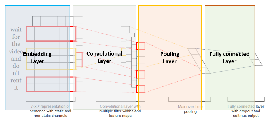
기본적인 구조입니다.
전처리를 진행해야죠
# total text tokens
total_words = []
for words in words_list:
    total_words.extend(words)

from collections import Counter
c = Counter(total_words)

# 빈도를 기준으로 상위 10000개의 단어들만 선택
max_features = 10000
common_words = [word for word, count in c.most_common(max_features)]

print(common_words.index('행'))
print(common_words[248])
토큰화해서 제일 많이 나온 단어 10000개만 사용할 겁니다.
확인해보면 행이란 단어는 248번째에 있는 것을 확인할 수 있습니다.
이제 가지고 있는 토큰화된 데이터를 인덱스로 하기 전에 데이터와 인덱스 1대 1 매칭을 하고, 그걸 돌리기 위한 사전 작업을 해둡니다.
# 각 단어에 대해서 index 생성하기
words_dic = {} # 각 단어가 하나의 인덱스를 가지도록
#Write your code
words_dic = {word: index for index, word in enumerate(common_words, start=1)}


# 각 index에 대해서 단어 기억하기
#Write your code
index_word = {index: word for word, index in words_dic.items()}


print(words_dic.get('영화',"aweg"))
print(words_dic.get('awe',0)) # 없는 값에선 0을 출력하게 만들었다.
print(index_word.get(1,"awer"))
그럼 이제 인덱스화를 진행합니다.
# 각 문서를 상위 10000개 단어들에 대해서 index 번호로 표현하기
# [['ㄷㅁㅈㅎ','ㅈㅁㅎㅁㅈㄷ','ㅁㅈㄷㅎㅁㅈ','ㅁㅈㄷㅎㅁ'...]...]
# [[1,2,3,4...]......]
filtered_indexed_words = []
#Write your code
filtered_indexed_words = [[words_dic.get(word, 0) for word in sentence] for sentence in words_list]
print(filtered_indexed_words[:7])
이제 여기선 인풋의 길이를 고정해줘야 하기 때문에 패딩을 집어 넣어야 합니다
여기서 평균 길이가 대략 11.7정도 되기 때문에 문장은 최대 14토큰만 유지 되도록 했습니다.
from tensorflow.keras.preprocessing import sequence
from tensorflow.keras.utils import to_categorical

#Write your code
# 토큰의 길이가 문장의 길이마다 다르기 때문에 가장 긴 값이 무엇인지 체크!
max_len = 0
total = 0
for x in filtered_indexed_words:
    total = total + len(x)
    if len(x) > max_len:
        max_len = len(x)

print(max_len) # 보통은 맥스 값으로 패딩한다. -> 모든 문장의 길이를 맥스로 맞춰준다.
# 2.1 X - input data 처리 (text tokens id_index to padded X)
max_len = 14
x_data = sequence.pad_sequences(filtered_indexed_words, maxlen=max_len)  # 대부분이 max_len보다 짧다 -> 20으로 맞춘다.

# 2.2 y - label data 처리 (one_hot_encoded y)
y_data = to_categorical(labels)
print(x_data[:7])
print(y_data[:7])
이제 train, test 데이터 셋을 나눠줍니다.
from sklearn.model_selection import train_test_split
#Write your code
# 2.3 Train / Test Split
x_train, x_test, y_train, y_test = train_test_split(x_data, y_data, test_size=0.1, random_state=42)

# 결과 확인
print("훈련 세트 크기:", x_train.shape, y_train.shape)
print("테스트 세트 크기:", x_test.shape, y_test.shape)
from tensorflow.keras import layers
from tensorflow.keras import models
from keras.regularizers import l2

model = models.Sequential() # 시퀀스의 형태로 변형한다. 뒤 이어 레이어를 추가해주낟.

# embedding layer 1000*256 *300
model.add(layers.Embedding(max_features, 256, input_shape=(max_len,))) # 전체 단어 수, 임베딩 레이어 차원, 인풋 차원(패딩을 한 이유)
#convolution layer
model.add(layers.Conv1D(256, 5, strides=1, padding='same'))
model.add(layers.BatchNormalization())
model.add(layers.Activation('relu'))
model.add(layers.Conv1D(256, 5, strides=1, padding='same'))
model.add(layers.BatchNormalization())
model.add(layers.Activation('relu'))
model.add(layers.MaxPool1D(2))


model.add(layers.Conv1D(512, 3, strides=1, padding='same'))
model.add(layers.BatchNormalization())
model.add(layers.Activation('relu'))

model.add(layers.Conv1D(512, 3, strides=1, padding='same'))
model.add(layers.BatchNormalization())
model.add(layers.Activation('relu'))
model.add(layers.MaxPool1D(2))


# FCN with Batch Normalization and ReLU
model.add(layers.Flatten())
model.add(layers.Dropout(0.2))

model.add(layers.Dense(256, kernel_regularizer=l2(0.1)))
model.add(layers.BatchNormalization())
model.add(layers.Activation('relu'))
model.add(layers.Dropout(0.2))

model.add(layers.Dense(32, kernel_regularizer=l2(0.1)))
model.add(layers.BatchNormalization())
model.add(layers.Activation('relu'))
model.add(layers.Dropout(0.2))

model.add(layers.Dense(2, activation='softmax'))

model.summary()
#Write your code - model build
모델은 단순하게부터 엄청 복잡하게 다 만들어 봤는데 계속 오버피팅이....
데이터도 많은데 왜 이런건진....
from tensorflow.keras.callbacks import EarlyStopping
from tensorflow.keras.callbacks import ModelCheckpoint
from tensorflow.keras.optimizers import RMSprop, Adam # you can add more optimizers

#Write your code - model setting
# early stopping 적용
es = EarlyStopping(monitor='val_loss', mode='min', verbose=1, patience=9)

# local에 저장하고 싶을 경우 이용
checkpoint_filepath = './temp/checkpoint.weights.h5'
mc = ModelCheckpoint(checkpoint_filepath, monitor='val_loss', mode='min', save_weights_only=True, save_best_only=True)

# optimizer에 필요한 옵션 적용
# loss와 평가 metric 적용

#model.compile(optimizer=RMSprop(learning_rate=0.001), loss='binary_crossentropy', metrics=['accuracy'])
model.compile(optimizer=Adam(learning_rate=0.001), loss='binary_crossentropy', metrics=['accuracy'])
저장하는 코드도 작성해주고, 빨리 멈출 수 있는 코드도 추가!
#Write your code - model training
#history = model.fit(x_train, y_train, epochs=20, batch_size=256, validation_split=0.2, callbacks=[es])
history = model.fit(x_train, y_train, epochs=20, batch_size=1024, validation_split=0.1,callbacks= [mc,es])
학습은 GPU 사용하면 엄청 금방 끝나더라고여
import matplotlib.pyplot as plt
plt.plot(history.history['loss'])
plt.plot(history.history['val_loss'])
plt.ylim(0,1)
plt.xlabel('epoch')
plt.ylabel('loss')
plt.legend(['train','val'])
plt.show()
엄청난 오버피팅 그래프가 나오게 됩니다...
test_loss, test_acc = model.evaluate(x_test,y_test)

print("Loss:", test_loss)
print("Accuracy:", test_acc)


model.load_weights(checkpoint_filepath)
test_loss, test_acc = model.evaluate(x_test,y_test)
print("Loss:", test_loss)
print("Accuracy:", test_acc)
모델 평가하기....
이렇게 마무리가 되었습니다...... 오버피팅 살려줘...
728x90
'인공지능 > 자연어 처리' 카테고리의 다른 글
| 자연어 이해 NLU - Relation Extraction Task 관계 추출 (0) | 2024.04.11 |
|---|---|
| 자연어 처리 온라인 강의 - Machine Translation with RNN (0) | 2024.04.10 |
| 자연어 이해 - 요약 TASK (0) | 2024.04.04 |
| 자연어 이해 - 자연어 추론 TASK (0) | 2024.04.04 |
| 자연어 이해 NLU- 감정 분석 Sentiment Analysis Task (0) | 2024.04.01 |