728x90
728x90
import numpy as np
import matplotlib.pyplot as plt
# ==================== Load Data ====================
# The first two columns contains the exam scores and the third column
# contains the label.
from google.colab import drive
drive.mount('/content/drive')
data = np.loadtxt('/content/drive/MyDrive/Colab Notebooks/ex2data2.txt', delimiter=',')
data = np.array(data)
X = data[:,0:2]
y = data[:,2:3]
# 이전 plotData 함수
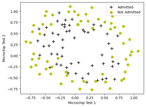
def plotData(X, y):
pos = np.where(y==1)
neg = np.where(y==0)
plt.figure()
# YOUR CODE HERE
plt.scatter(X[pos,0],X[pos,1],marker='+',c='black',s=80,label='Admitted')
plt.scatter(X[neg,0],X[neg,1],marker='o',c='y',s=50,label='Not Admitted')
plotData(X, y)
# Labels and Legend
plt.xlabel('Microchip Test 1')
plt.ylabel('Microchip Test 2')
plt.legend()
plt.show()
Mounted at /content/drive
# ======================= Part 1: Regularized Logistic Regression =======================
# In this part, you are given a dataset with data points that are not
# linearly separable. However, you would still like to use logistic
# regression to classify the data points.
# To do so, you introduce more features to use -- in particular, you add
# polynomial features to our data matrix (similar to polynomial
# regression).
# Add Polynomial Features
# Note that mapFeature also adds a column of ones for us, so the intercept
# term is handled
# 제공되는 함수
def mapFeature(X1, X2):
degree = 6
X1 = X1.reshape(-1,1)
X2 = X2.reshape(-1,1)
out = np.ones(np.size(X1[:,0]))
for i in range(1, degree + 1):
for j in range(i + 1):
new_feature = (X1**(i-j)) * (X2**j)
out = np.column_stack((out, new_feature))
return out
X = mapFeature(X[:,0], X[:,1]);
initial_theta = np.zeros((X.shape[1],1))
lambda_1 = 1
# 이전 sigmoid 함수
def sigmoid(z):
return 1/(1+np.e**(-z));
def sigmoid(z):
# YOUR CODE HERE
g = 1 / (1 + np.exp(-z))
return g
def costFunctionReg(theta, X, y, lambda_1):
# YOUR CODE HERE
m = len(y)
h = sigmoid(X@theta)
print(h.shape)
print(y.shape)
J= (-1/m) *(y.T@np.log(h)+(1-y).T@np.log(1-h)) + lambda_1/2/m*((np.sum(theta*theta)) -theta[0]*theta[0])
grad = (1/m*(X.T@(h-y))) + lambda_1/m*theta
grad[0] = grad[0] - (lambda_1/m) * theta[0]
return J, grad
cost, grad = costFunctionReg(initial_theta, X, y, lambda_1)
print('Cost at initial theta (zeros): ', cost)
print('Expected cost (approx): 0.693')
print('Gradient at initial theta (zeros) - first five values only:')
print(grad[0:5].reshape(-1,1))
print('Expected gradients (approx) - first five values only:')
print(' 0.0085\n 0.0188\n 0.0001\n 0.0503\n 0.0115')
(118, 1) (118, 1) Cost at initial theta (zeros): [[0.69314718]] Expected cost (approx): 0.693 Gradient at initial theta (zeros) - first five values only: [[8.47457627e-03] [1.87880932e-02] [7.77711864e-05] [5.03446395e-02] [1.15013308e-02]] Expected gradients (approx) - first five values only: 0.0085 0.0188 0.0001 0.0503 0.0115
# Compute and display cost and gradient
# with all-ones theta and lambda = 10
test_theta = np.ones((X.shape[1],1));
[cost, grad] = costFunctionReg(test_theta, X, y, 10);
print('Cost at test theta (with lambda = 10): ', cost)
print('Expected cost (approx): 3.16')
print('Gradient at test theta - first five values only:')
print(grad[0:5].reshape(-1,1))
print('Expected gradients (approx) - first five values only:')
print(' 0.3460\n 0.1614\n 0.1948\n 0.2269\n 0.0922')
Cost at test theta (with lambda = 10): [[3.16450933]] Expected cost (approx): 3.16 Gradient at test theta - first five values only: [[0.34604507] [0.16135192] [0.19479576] [0.22686278] [0.09218568]] Expected gradients (approx) - first five values only: 0.3460 0.1614 0.1948 0.2269 0.0922
## ============= Part 2: Regularization and Accuracies =============
# Optional Exercise:
# In this part, you will get to try different values of lambda and
# see how regularization affects the decision coundart
# Try the following values of lambda (0, 1, 10, 100).
# How does the decision boundary change when you vary lambda? How does
# the training set accuracy vary?
# Set options for fminunc in python using scipy minimize
from scipy.optimize import minimize
# Initialize fitting parameters
initial_theta = np.zeros((X.shape[1], 1));
# Set regularization parameter lambda to 1 (you should vary this)
lambda_2 = 1
# Set Options
options = {'disp': True, 'maxiter': 400}
# Optimize
initial_theta = initial_theta.ravel()
y=y.flatten()
result = minimize(fun=costFunctionReg, x0=initial_theta, args=(X, y, lambda_2),
method='TNC', jac=True, options=options)
theta = result.x
cost = result.fun
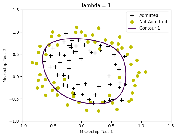
# 제공되는 함수
def plotDecisionBoundary(theta, X, y):
plotData(X[:,1:3], y)
if X.shape[1] <= 3:
plot_x = [np.min(X[:,1])-2, np.max(X[:,1])+2]
plot_y = (-1./theta[2]) * (theta[1] * np.array(plot_x) + theta[0])
plt.plot(plot_x, plot_y, '-', label='Decision boundary')
else:
u = np.linspace(-1, 1.5, 50)
v = np.linspace(-1, 1.5, 50)
z = np.zeros((len(u), len(v)))
for i in range(len(u)):
for j in range(len(v)):
z[i, j] = np.dot(mapFeature(u[i], v[j]), theta)
contour_plt = plt.contour(u, v, z.T, [0], linewidths=2)
h1,l1 = contour_plt.legend_elements()
handles, labels = plt.gca().get_legend_handles_labels()
handles += [h1[0]]
labels += ['Contour 1']
plt.legend(handles, labels)
plt.title('lambda = ' + str(lambda_2))
plt.xlabel('Microchip Test 1')
plt.ylabel('Microchip Test 2')
plt.show()
plotDecisionBoundary(theta, X, y)
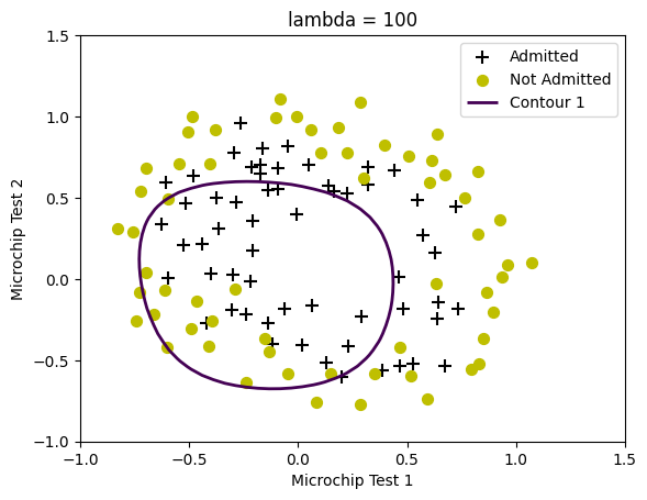
lambda_2 = 100
# Set Options
options = {'disp': True, 'maxiter': 400}
# Optimize
initial_theta = initial_theta.ravel()
y=y.flatten()
result = minimize(fun=costFunctionReg, x0=initial_theta, args=(X, y, lambda_2),
method='TNC', jac=True, options=options)
theta = result.x
cost = result.fun
plotDecisionBoundary(theta, X, y)
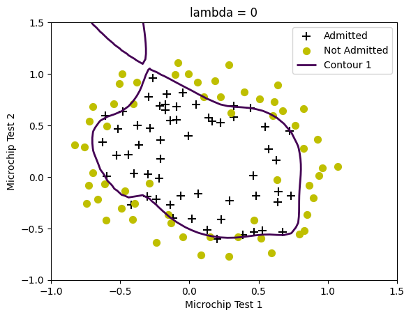
lambda_2 = 0
# Set Options
options = {'disp': True, 'maxiter': 400}
# Optimize
initial_theta = initial_theta.ravel()
y=y.flatten()
result = minimize(fun=costFunctionReg, x0=initial_theta, args=(X, y, lambda_2),
method='TNC', jac=True, options=options)
theta = result.x
cost = result.fun
plotDecisionBoundary(theta, X, y)
728x90
'인공지능 > 공부' 카테고리의 다른 글
| FCN quiz (0) | 2023.11.16 |
|---|---|
| FCN - tensorflow (0) | 2023.11.15 |
| 1 vs all classification (0) | 2023.11.15 |
| logistic Regression (0) | 2023.11.13 |
| Linear regression 1 (0) | 2023.11.13 |