728x90
728x90
import numpy as np
import matplotlib.pyplot as plt
from google.colab import drive
drive.mount('/content/drive')
# ==================== Load Data ====================
# The first two columns contains the exam scores and the third column
# contains the label.
data = np.loadtxt('/content/drive/MyDrive/Colab Notebooks/ex2data1.txt', delimiter=',')
data = np.array(data)
X = data[:,0:2]
y = data[:,2:3]
# ======================= Part 1: Plotting =======================
# We start the exercise by first plotting the data to understand the
# the problem we are working with.
print('Plotting data with + indicating (y = 1) examples and o '\
'indicating (y = 0) examples.\n');
def plotData(X, y):
pos = np.where(y==1)
neg = np.where(y==0)
plt.figure()
plt.scatter(X[pos,0],X[pos,1],marker='+',c='black',s=80,label='Admitted')
plt.scatter(X[neg,0],X[neg,1],marker='o',c='y',s=50,label='Not Admitted')
plotData(X, y)
plt.xlim(30,100)
plt.ylim(30,100)
# Labels and Legend
plt.xlabel('Exam 1 score')
plt.ylabel('Exam 2 score')
plt.legend()
plt.show()
Plotting data with + indicating (y = 1) examples and o indicating (y = 0) examples.
# =================== Part 2: Compute Cost and Gradient ===================
# In this part of the exercise, you will implement the cost and gradient
# for logistic regression. You neeed to complete the code in
# Setup the data matrix appropriately, and add ones for the intercept term
m,n = X.shape
# Add intercept term to x and X_test
X = np.column_stack((np.ones(m), X))
# Initialize fitting parameters
initial_theta = np.zeros((n + 1, 1))
# Compute and display initial cost and gradient
def sigmoid(z):
return 1/(1+np.e**(-z));
def costFunction(theta, X, y):
m = len(y)
h = sigmoid(X@theta)
J= (-1/m) *(y.T@np.log(h)+(1-y).T@np.log(1-h))
grad = (1/m*(X.T@(h-y))).reshape(-1)
#grad.flatten()
return J, grad
# Compute and display initial cost and gradient
cost, grad = costFunction(initial_theta, X, y)
print('Cost at initial theta (zeros):', cost)
print('Expected cost (approx): 0.693')
print('Gradient at initial theta (zeros): ')
print(grad)
print('Expected gradients (approx):\n -0.1000\n -12.0092\n -11.2628\n')
Cost at initial theta (zeros): [[0.69314718]] Expected cost (approx): 0.693 Gradient at initial theta (zeros): [ -0.1 -12.00921659 -11.26284221] Expected gradients (approx): -0.1000 -12.0092 -11.2628
# Compute and display cost and gradient with non-zero theta
test_theta = np.array([[-24], [0.2], [0.2]])
cost, grad = costFunction(test_theta, X, y)
print('\nCost at test theta:', cost)
print('Expected cost (approx): 0.218')
print('Gradient at test theta: ')
print(grad.reshape(-1,1))
print('Expected gradients (approx):\n 0.043\n 2.566\n 2.647\n')
print('Program paused. Press enter to continue.')
Cost at test theta: [[0.21833019]] Expected cost (approx): 0.218 Gradient at test theta: [[0.04290299] [2.56623412] [2.64679737]] Expected gradients (approx): 0.043 2.566 2.647 Program paused. Press enter to continue.
# =================== Part 3: Optimizing using minimize in python ===================
# In this exercise, you will use a function (minimize) to find the
# optimal parameters theta.
from scipy.optimize import minimize
options = {'disp': True, 'maxiter': 400}
# Add intercept term to x and X_test
initial_theta = initial_theta.ravel()
y=y.flatten()
result = minimize(fun=costFunction, x0=initial_theta, args=(X, y),method='TNC', jac=True, options=options)
theta = result.x
cost = result.fun
# Print theta to screen
print('Cost at theta found by fminunc: ', cost);
print('Expected cost (approx): 0.203');
print('theta: ');
print(theta.reshape(-1,1));
print('Expected theta (approx):');
print(' -25.161\n 0.206\n 0.201\n');
Cost at theta found by fminunc:  0.20349770158947478
Expected cost (approx): 0.203
theta:
[[-25.16131856]
 [  0.20623159]
 [  0.20147149]]
Expected theta (approx):
 -25.161
 0.206
 0.201
<ipython-input-23-35c8161c9a44>:11: OptimizeWarning: Unknown solver options: maxiter
  result = minimize(fun=costFunction, x0=initial_theta, args=(X, y),method='TNC', jac=True, options=options)
# 제공되는 함수
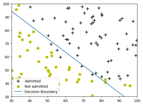
def plotDecisionBoundary(theta, X, y):
plotData(X[:,1:3], y);
if X.shape[1] <= 3:
# Only need 2 points to define a line, so choose two endpoints
plot_x = [np.min(X[:,1])-2, np.max(X[:,1])+2]
# Calculate the decision boundary line
plot_y = (-1./theta[2]) * (theta[1] * np.array(plot_x) + theta[0])
# Plot, and adjust axes for better viewing
plt.plot(plot_x, plot_y, '-')
# Legend, specific for the exercise
plt.legend(['Admitted', 'Not admitted', 'Decision Boundary'])
plt.axis([30, 100, 30, 100])
plt.show()
else :
# Here is the grid range
u = np.linspace(-1, 1.5, 50)
v = np.linspace(-1, 1.5, 50)
z = np.zeros((len(u), len(v)))
# Define mapFeature function or ensure it's already defined.
# Assuming mapFeature returns a 1-D array
def mapFeature(X1, X2):
degree = 6
out = np.ones(np.size(X1[:,0]))
for i in range(1, degree + 1):
for j in range(i + 1):
new_feature = (X1**(i-j)) * (X2**j)
out = np.column_stack((out, new_feature))
return out
# Evaluate z = theta*x over the grid
for i in range(len(u)):
for j in range(len(v)):
z[i, j] = np.dot(mapFeature(u[i], v[j]), theta)
# Plot z = 0
# Notice you need to specify the range [0, 0]
plt.contour(u, v, z.T, [0], linewidths=2)
plt.show()
plotDecisionBoundary(theta, X, y)
# =================== Part 4: Predict and Accuracies ===================
# After learning the parameters, you'll like to use it to predict the outcomes
# on unseen data. In this part, you will use the logistic regression model
# to predict the probability that a student with score 45 on exam 1 and
# score 85 on exam 2 will be admitted.
# Furthermore, you will compute the training and test set accuracies of
# our model.
# Your task is to complete the code in predict.m
# Predict probability for a student with score 45 on exam 1
# and score 85 on exam 2
pred_X = np.array([1, 45, 85]).reshape(1,-1)
prob = sigmoid(pred_X.dot(theta))
print('For a student with scores 45 and 85, we predict an admission ' \
'probability of ', prob);
print('Expected value: 0.775 +/- 0.002\n\n');
# Compute accuracy on our training set
def predict(theta, X):
p = sigmoid(np.sum(X*theta,axis=1))
for i in range(p.size):
if p[i]>=0.5:
p[i]=1
else:
p[i]=0
return p
p = predict(theta, X);
y = y.reshape(-1)
accuracy = np.mean(p == y) * 100
print('Train Accuracy: ', accuracy)
print('Expected accuracy (approx): 89.0')
For a student with scores 45 and 85, we predict an admission probability of [0.77629062] Expected value: 0.775 +/- 0.002 Train Accuracy: 89.0 Expected accuracy (approx): 89.0
728x90
'인공지능 > 공부' 카테고리의 다른 글
| FCN quiz (0) | 2023.11.16 |
|---|---|
| FCN - tensorflow (0) | 2023.11.15 |
| 1 vs all classification (0) | 2023.11.15 |
| Logistic regression + regularized (1) | 2023.11.14 |
| Linear regression 1 (0) | 2023.11.13 |