728x90
728x90
import numpy as np
import matplotlib.pyplot as plt
output
Running warmUpExercise ...
5x5 Identity Matrix:
array([[1., 0., 0., 0., 0.],
       [0., 1., 0., 0., 0.],
       [0., 0., 1., 0., 0.],
       [0., 0., 0., 1., 0.],
       [0., 0., 0., 0., 1.]])
# ======================= Part 2: Plotting =======================
print('Plotting Data ...')
from google.colab import drive
drive.mount('/content/drive')
data = np.loadtxt('/content/drive/MyDrive/Colab Notebooks/ex1data1.txt', delimiter=',')
data = np.array(data)
X = data[:,0]
y = data[:,1]
m = len(y)
plt.figure()
plt.scatter(X,y)
# =================== Part 3: Cost and Gradient descent ===================
X = np.column_stack((np.ones(m), X))
theta = np.zeros(2)
Plotting Data ...
Drive already mounted at /content/drive; to attempt to forcibly remount, call drive.mount("/content/drive", force_remount=True).

# Some gradient descent settings
iterations = 1500
alpha = 0.01
print('Testing the cost function ...')
# compute and display initial cost
def computeCost(X, y, theta):
# YOUR CODE HERE
m = len(y)
J = np.sum((X.dot(theta) - y) ** 2) / (2 * m)
return J
J = computeCost(X, y, theta)
print('With theta = [0 ; 0] \nCost computed = ', J)
print('Expected cost value (approx) 32.07')
Testing the cost function ... With theta = [0 ; 0] Cost computed = 32.072733877455676 Expected cost value (approx) 32.07
# further testing of the cost function
J = computeCost(X, y, [-1, 2])
print('With theta = [-1 ; 2] \n Cost computed = ', J)
print('Expected cost value (approx) 54.24')
output
With theta = [-1 ; 2]
 Cost computed =  54.24245508201238
Expected cost value (approx) 54.24
# run gradient descent
theta = [-50,-50]
print('Running Gradient Descent ...')
def gradientDescent(X, y, theta, alpha, iterations):
# YOUR CODE HERE
m = len(y)
J_record = []
for _ in range(iterations):
gradJ = (X.T.dot(X.dot(theta) - y))/m
theta = theta - alpha * gradJ
J_record.append(computeCost(X, y, theta))
return theta, J_record
theta, J_record = gradientDescent(X, y, theta, alpha, iterations)
plt.figure()
plt.plot(J_record)
print('Theta found by gradient descent:')
print(theta)
print('Expected theta values (approx)')
print('-3.6303, 1.1664')
J = computeCost(X, y, theta)
print('J =',J)
Running Gradient Descent ...
Theta found by gradient descent:
[-6.60389588  1.46509317]
Expected theta values (approx)
-3.6303,  1.1664
J = 5.144644149724434

# Plot the linear fit
plt.figure()
plt.scatter(X[:,1], y, label='Training data')
plt.plot(X[:,1], X.dot(theta), label = 'Linear regression')
plt.legend()
plt.show()

# Predict values for population sizes of 35,000 and 70,000
predict1 = np.array([1, 3.5]).dot(theta)
print('For population = 35,000, we predict a profit of ',predict1*10000)
predict2 = np.array([1, 7]).dot(theta)
print('For population = 70,000, we predict a profit of ',predict2*10000)
For population = 35,000, we predict a profit of 390129.08230406477 For population = 70,000, we predict a profit of 221840.19017197358
# ============= Part 4: Visualizing J(theta_0, theta_1) =============
print('Visualizing J(theta_0, theta_1) ...')
# Grid over which we will calculate J
theta0_vals = np.linspace(-10, 10, 100)
theta1_vals = np.linspace(-1, 4, 100)
# initialize J_vals to a matrix of 0's
J_vals = np.zeros((len(theta0_vals), len(theta1_vals)))
# Fill out J_vals
for i in range(len(theta0_vals)):
for j in range(len(theta1_vals)):
t = np.array([theta0_vals[i], theta1_vals[j]])
J_vals[i,j] = computeCost(X, y, t)
J_vals = J_vals.T
fig = plt.figure()
ax = fig.add_subplot(111, projection='3d')
theta0_vals, theta1_vals = np.meshgrid(theta0_vals, theta1_vals)
ax.plot_surface(theta0_vals, theta1_vals, J_vals, cmap='viridis')
ax.set_xlabel('theta_0')
ax.set_ylabel('theta_1')
ax.set_zlabel('J(\theta_0, \theta_1)')
plt.show()
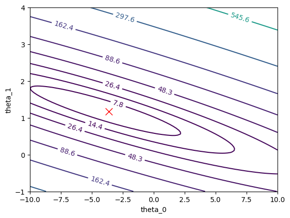
# Contour plot
plt.figure()
contour = plt.contour(theta0_vals, theta1_vals, J_vals, levels=np.logspace(-2, 3, 20))
plt.clabel(contour, inline=1, fontsize=10)
plt.xlabel('theta_0')
plt.ylabel('theta_1')
plt.plot(theta[0], theta[1], 'rx', markersize=10, linewidth=2)
plt.show()
/usr/local/lib/python3.10/dist-packages/IPython/core/pylabtools.py:151: UserWarning: Glyph 9 (	) missing from current font.
  fig.canvas.print_figure(bytes_io, **kw)

728x90
'인공지능 > 공부' 카테고리의 다른 글
| FCN quiz (0) | 2023.11.16 |
|---|---|
| FCN - tensorflow (0) | 2023.11.15 |
| 1 vs all classification (0) | 2023.11.15 |
| Logistic regression + regularized (1) | 2023.11.14 |
| logistic Regression (0) | 2023.11.13 |