딥러닝 공부하기 2

인공지능/공부

딥러닝 공부하기 2

이게될까 2025. 7. 2. 02:59

728x90

6강 - CNN

📌 개요: Convolutional Neural Networks (CNNs)

CNN은 주로 이미지 분류를 위한 특수한 형태의 피드포워드 신경망이며, 입력의 공간적 정보(spatial information) 를 활용한다.
전통적인 완전연결신경망(Fully Connected Network)에 비해 매개변수 수가 현저히 적고, 학습 효율이 높다.

🧱 핵심 구성 요소

1. Convolution Layer (합성곱 층)

입력 텐서에 필터(커널) 를 슬라이딩하여, 지역적인 특징을 추출.
연산 방식은 입력과 필터의 원소별 곱의 합 (weighted sum) 을 통해 특징 맵(feature map)을 생성.
Stride, Padding 등의 하이퍼파라미터 조절로 출력 크기 및 정보 손실 제어 가능.

🔸 Multi-channel 입력

컬러 이미지(RGB 등)는 다중 채널 입력으로 처리되며, 각 채널에 대해 별도의 필터 연산 수행.
CNN은 다중 채널 입력을 하나의 통합된 출력 특징 맵으로 계산 가능.

2. Pooling Layer (풀링 층)

지역적으로 특징을 요약하여 공간 크기 축소 및 연산 효율 향상.
대표적인 방식:
- Max Pooling: 지역 내 최댓값 추출 → 엣지 등 뚜렷한 특징 유지
- Average Pooling: 지역 평균값 추출
Downsampling 역할을 통해 과적합 완화 및 연산량 감소.

3. Fully-Connected Layer (완전 연결층)

마지막 단계에서 추출된 고수준 특징들을 벡터화하고, 클래스 확률 등의 최종 예측을 수행.
Convolution + Pooling으로 추출한 특징을 벡터(flatten) 형태로 연결하여 classification 등 downstream task 수행.

🔄 학습 구조

1. Forward Propagation

입력 → 합성곱 → 풀링 → 완전연결 → 출력까지 흐름에 따라 출력 계산.

2. Backward Propagation

손실함수 기반 오차를 바탕으로 chain rule을 통해 가중치 업데이트 (역전파).

🧠 CNN의 표현력: 계층적 표현 (Hierarchical Representation)

초기 층은 에지나 패턴 등 저수준 특징 추출
심층 층으로 갈수록 물체의 구조, 형태 등 고수준 의미적 특징 학습
특징 표현이 점진적으로 복잡해지는 계층적 특징 추출 구조

📈 주요 CNN 모델 아키텍처

모델	주요 특징	논문
LeNet	평균 풀링, 시그모이드/탄젠트 비선형성	LeCun et al., 1998
AlexNet	ReLU, 드롭아웃, 데이터 증강 사용. 대규모 ImageNet 분류	Krizhevsky et al., 2012
VGGNet	3×3 필터 사용으로 깊이 확장, 구조 단순화	Simonyan et al., 2014
GoogleNet (Inception)	다양한 크기의 필터를 병렬로 구성한 Inception 모듈	Szegedy et al., 2014
ResNet	Residual connection(skip connection)을 통한 gradient 흐름 보존	He et al., 2016
SENet	Squeeze-and-Excitation 블록을 통해 채널 간 중요도 재조정	Hu et al., 2017

🧩 CNN의 강점 요약

공간적 계층 구조를 기반으로, 고차원의 복잡한 이미지 특징을 효과적으로 추출
적은 파라미터 수로도 효율적 학습 가능
다양한 구조적 변형과 조합이 가능하여 표현력과 일반화 성능을 모두 확보

주요 초점은 합성곱 연산의 구체적 동작 방식, CNN의 계층 구조의 실제 구현 원리, 각 CNN 모델의 발전 흐름, 그리고 성능 향상을 위한 구조적 기법에 있습니다.

📌 Convolutional Neural Networks (CNN)의 세부 구조 및 발전

1. 🔍 합성곱 연산의 구체적 원리

필터(커널)는 작은 행렬 형태로, 입력 이미지와 원소별 곱 후 합산 (element-wise product + sum) 하는 방식으로 작동함.
스트라이드(stride)와 패딩을 조정하여 출력 크기를 조절할 수 있으며, 입력 이미지 전체를 스캔하며 특징 맵을 생성.
예시 필터:
- 대각선 값만 1이고 나머지는 -1인 필터는 선(line) 검출기로 작동함.
- 다른 방향의 선을 검출하는 다양한 필터 조합 가능.

2. 🎨 다채널 입력 및 출력 처리

컬러 이미지와 같이 RGB 채널을 가진 입력에도 각각의 채널에 대해 필터를 적용하고, 그 결과를 합산하여 출력 생성.
다채널 필터와 다채널 출력은 다음 합성곱 계층의 입력으로 이어져, 깊은 네트워크 구성 가능.

3. 🧊 풀링(Pooling)의 역할과 종류

Max Pooling: 각 지역에서 최대값 추출 → 뚜렷한 특징 유지
Average Pooling: 각 지역의 평균값 → 부드러운 축소 효과
주요 역할:
- 차원 축소 (downsampling) 을 통한 연산 효율화
- 과적합 감소 및 위치 불변성 (translation invariance) 확보

🧠 CNN 모델의 계층적 구성

기본 구조: Convolution → Pooling → Convolution → Pooling → Fully Connected → Output
각 계층은 점차 더 복잡한 표현 (hierarchical feature representation) 을 학습
- 초기: 엣지, 선
- 중간: 패턴, 텍스처
- 후기: 개체의 의미적 구조

🧱 대표적 CNN 모델들의 진화

모델	주요 특징 및 구조적 차별성
LeNet (1998)	초기 CNN. 손글씨 인식용. 단순한 2개 Conv+Pooling → FC 구조
AlexNet (2012)	대규모 필터(60M 파라미터), ReLU, Dropout, Data Augmentation 적용
VGGNet (2014)	작은 필터 (3×3) 를 깊이 있게 누적 → 단순 구조로 깊이 확보
GoogLeNet (Inception, 2014)	다양한 크기의 필터를 병렬로 처리하는 Inception 모듈 도입
ResNet (2015)	Residual connection (skip connection) 으로 gradient 흐름 문제 해결
SENet (2017)	채널 간 중요도를 반영하는 Squeeze-and-Excitation 블록 사용

🔧 모델 성능 향상을 위한 핵심 구조적 아이디어

✅ Residual Connection (ResNet)

정보 흐름을 우회(bypass) 할 수 있는 경로를 추가
문제 해결:
- 입력 정보가 깊은 층까지 전달되지 않는 문제
- 역전파에서 gradient가 사라지는 문제 (vanishing gradient)
결과적으로 더 깊은 모델도 안정적으로 학습 가능

✅ Squeeze-and-Excitation (SE) Block

각 채널의 global 정보를 압축(squeeze)하고, 중요도를 학습하여 (excitation) 채널별 가중치를 조정
구성:
- Global Average Pooling → 각 채널별 통계 정보 추출
- 2개 FC layer → 중요도 weight 학습
- 입력 feature map에 weight를 곱하여 채널 선택적 강조

📊 ImageNet Challenge와 성능 지표

ImageNet: 1,000개 클래스, 120만 개 학습 이미지
평가 방식: Top-5 Error
- 모델이 예측한 5개의 클래스 중 정답이 포함되면 정답으로 간주
CNN의 발전 흐름:
- 초기에는 인간보다 낮은 정확도 → ResNet 이후 인간보다 높은 성능 도달

🧩 요약

영역	내용 요약
합성곱	입력과 필터의 가중합으로 특징 추출
다채널 처리	RGB 등 멀티채널에 대한 병렬 필터 적용
풀링	지역 요약 (최댓값/평균값), 차원 축소
계층적 표현	저수준 → 고수준 특징 추출
대표 모델	LeNet, AlexNet, VGG, GoogLeNet, ResNet, SENet
구조적 개선	Residual, Inception, SE Block으로 성능 개선

📌 CNN (Convolutional Neural Network) 심화 개요

1. 🎯 CNN의 핵심 철학: 로컬 연결성과 계층적 학습

CNN은 이미지 내 지역적 패턴 (local pattern) 을 효과적으로 감지하고, 이들을 계층적으로 결합해 복잡한 구조를 인식하도록 설계된 신경망이다.

합성곱층: 로컬 필터(커널)를 이용해 엣지, 코너, 텍스처 등을 추출하는 학습 가능한 특징 감지기로 동작
가중치 공유 (weight sharing) 와 로컬 연결 (local connectivity) 을 통해 매우 적은 파라미터로 고차원 시각 정보 학습 가능

2. 🧮 합성곱 연산의 동작 세부

필터는 입력 이미지와 원소별 곱셈 후 합산 (weighted sum)을 수행하며, 이는 마치 고전적인 커널 기반 edge detector와 유사
필터의 이동 간격은 stride로 조절되며, 이미지 경계에서 정보 손실을 줄이기 위한 패딩(padding) 기법도 자주 함께 사용
이 연산이 반복되면 특징 맵(feature map) 이 생성되며, 각 맵은 특정 패턴(예: 수직선, 대각선 등)에 강하게 반응

3. 🌈 다채널 입력 및 출력 처리

RGB 이미지처럼 다채널 입력은 각 채널에 대해 필터를 적용하고, 그 결과를 채널 축을 따라 합산하여 하나의 출력으로 만듦
여러 개의 필터를 병렬로 적용하면, 출력도 다채널화되어 다음 층에서 더욱 복잡한 패턴 학습 가능
이러한 구조는 다차원 색상/텍스처 조합을 학습하는 데 핵심적임

4. 📉 풀링(Pooling)의 원리와 기능

합성곱 층 이후, 공간 정보를 압축하면서도 주요 특징을 보존하기 위해 사용됨
주요 방식:
- Max Pooling: 가장 두드러진 특징 유지
- Average Pooling: 평균값을 통해 부드러운 요약
목적:
- 특징 추출의 위치 불변성 (translation invariance) 확보
- 차원 축소 및 연산량 감소, 과적합 방지

🏗️ CNN의 계층 구조와 학습 흐름

CNN은 다음과 같은 방식으로 계층적 표현 학습(hierarchical representation learning) 을 구현한다:

계층	학습 내용	의미
저층	엣지, 모서리 등 단순 시각 요소	로컬 감지
중층	텍스처, 반복 패턴 등	구조 인식
고층	객체 형태, 의미적 구성	고수준 인식

이러한 점진적 추상화는 복잡한 이미지도 점진적으로 이해하게 하는 핵심 원리다.

📚 주요 CNN 모델 및 아키텍처 진화

모델	핵심 구조	주요 혁신
LeNet	단순 2Conv + FC	초기 손글씨 인식 CNN
AlexNet	필터 수 대폭 증가, ReLU, Dropout	CNN 대중화, ImageNet 도약의 계기
VGGNet	3x3 작은 필터 반복으로 깊이 증가	단순하지만 강력한 구조로 대표됨
GoogLeNet	Inception 모듈 도입, 병렬 경로 구조	멀티스케일 특징 추출 효과
ResNet	Skip connection으로 정보/gradient 직접 전달	딥 네트워크의 학습 안정성 확보
SENet	채널 간 중요도 학습(Attention 기반)	정교한 특징 강조, 분류 성능 향상

🚀 구조적 혁신에 의한 성능 향상 요인

🔁 Residual Connection (ResNet)

깊은 신경망에서 입력 정보 손실과 기울기 소실 문제 발생
이를 해결하기 위해, 입력을 다음 층으로 직접 전달하는 스킵 경로(shortcut path) 도입
효과:
- 학습 초기에 gradient 흐름이 잘 유지되어 안정적 수렴 가능
- 100층 이상의 네트워크도 학습 가능

🎯 Squeeze-and-Excitation (SE) Block

각 채널의 중요도를 학습하여 중요한 특징만 강조
구성:
- Squeeze: Global Average Pooling → 채널 요약
- Excitation: 2개 FC Layer → 채널별 가중치 학습
- 출력: 원본 feature map × 중요도 weight → 정제된 표현
결과적으로 CNN이 불필요한 특징 억제, 의미 있는 특징 강조

🔍 실전적 통찰

통찰	설명
CNN은 효율적인 학습 구조이다	가중치 공유 및 로컬 연결성을 통해 연산량 절감
계층이 깊어질수록 추상화 수준이 증가한다	구조적 패턴 → 형태 → 의미로 학습 전개
필터는 특징 감지기 역할을 한다	직접 학습되어 이미지 내 반복 구조를 감지
Residual, SE Block은 성능을 극적으로 향상시킨다	정보 흐름과 중요도 조절을 통해 네트워크 일반화 향상

🧾 정리

요소	설명
합성곱	지역 특징 추출, 파라미터 절감
다채널 필터링	RGB 및 다채널 대응, 표현력 강화
풀링	정보 요약 및 모델 경량화
계층적 표현	점진적 패턴 학습 구조
대표 모델	LeNet → AlexNet → VGG → GoogLeNet → ResNet → SENet
고급 기법	Residual, Inception, SE block 등

00:00:01 In the previous lecture, we learned that how we can well train our neural network. Now let's see one of special types of neural networks convolutional neural networks which is called as CNN. The convolutional neural networks is designed for image classification. So this is a special type of feed for neural networks. So the CNN use information of input with convolutional operations. One advantage of CNN is reducing the number of parameters by adopting the network architecture designed for vision

00:00:58 tasks. Conventional CNN consist of three different types of layers. The first one is convolution layer and next one is cooling layer. The final is fully connected layer. So now let's see them one by one. Let's first see what the convolution layer is. Actually the convolution operation or widely used in traditional machine learning for computer vision. Now let's suppose that you have this kind of input image and you will also have this kind of filters. You can also call it as kernel. Then let's first put the filter

00:02:02 to the left top input image like the lead box. Then please consider values in the filter as weight and the input is the data. Then you can weight the sum of this weight and data. Then you can perform element wise multiplication of each component and then sum them together for the output. So you will get the output value three for the first element. Now let's put the left box to right. In this example, I pushed the red box just one pixel. The stride will be one. Now let's perform the weighted sum

00:03:23 again for this input and the filter. And then we will get the different output value for the next elements. Now you can push the letter box to the next and next and next like this. So if you perform the same things recursively like this then the filters can the every values of input from left top corner to right down corner like this and according to their input we will get the weighted sum output like this. Now let's think about the role of the filter. In this example, you can simply see that only diagonal elements of the

00:04:30 filter have one value and other parts have minus one value. So the filter works like a line detector. Let's see the first case again. In the case you can also see the input has the same pattern like the filter. In this case we will have high output values like this. On the other hand, if we put the filter at this point, we will get the lower output value. So if we have this kind of line at input like filter, we will get a higher value. So this is a type of line detector. We can also have different types of

00:05:44 filters like this. If we scan the input by using the convolution operation with this filter then we will get the different output values like this. Then this filter will work like another line detector to find this kind of line. So you can use more filter to detect different types of input patterns. Please note that we only use very small number of ways compared to the previous fully connected neural networks. We can also use convolutional layer for multi- channelannel input. You may know that color images

00:06:48 consist of RGB channels. So we can also apply convolutional layers to color images input with multi- channelannel approaches. Moreover, the output of convolutional layers also consists of multi- channels. Previously we used two different types of filters filter one and filter two. So if we apply the filter one to input we get the output one and if we use filter two we can get the output too like this. Then each of the output becomes each channel and the multi- channelannel output becomes the multi- channelannel

00:07:46 inputs in the next convolutional layer. In the case of the multi- channelannel input, we can also use the multi- channelannel filters. So we can also apply the element wise multiplication for multi- channelannel input and multi- channelannel filters to generate the output. Now let's take about pooling layer. Actually pulling layer is very simple. So after the convolution layer we get the output like this and and let's perform pulling to this output. We will also perform convolution operations but in this case there is no

00:08:45 filter or weight. instead that we just extract max value from the input. So if we scan the input and extract max value recursively like this and like this we will get this kind of output that's all that is pulling player. So in the pooling layer we can extract max value or average value. So in the first case we will call it as max pooling and the next case we will call it as the average pooling. So let's think about the low of the pooling layer actually. So the pooling layer will perform the soft

00:09:54 sampling. So by using the pooling layer we can reduce the number of parameters to represent the image without change the objects. The last one is fully connected layer. The fully connected layer. Uh every element of the input will be vectorized. So just put the vector as input of fully connected neural network. So this is convolutional neural networks. In the CNN, we stack a pair of convolution and pooling layer like this. And then finally stack some fully connected layers to connect the input to

00:10:52 the output layer. So in world propagation we will estimate the output from the input according to our weights of the neural networks and then we will measure the loss between our estimation and the true output value. And based on the loss we will update the weight during back propagation. So this is examples of hierarchical representation of CNN. You can see that vectors of the lower layer it looks like very simple but when we go higher layer you can see that very complex and meaningful shapes or patterns of image

00:11:56 like this. Now let's see the different types of convolutional neural networks. The first one is ced as renet which is trained for handwrite document recognition. Since this is a very early CN model, it has a very simple structure. So it consists of two pair of convolutional and pooling layers and then it stack fully connected layers for character recognition. These are the results of the renet. So these are the input of the renet for digit four and in that case the renet will recognize the digit as

00:12:54 four. Also you can see that the renet will work for digit recognition even though there are some noises like this. After the renet, many advanced techniques for CNN are proposed in the MNET challeng. The challenge provide 1.2 million training samples with 1,000 object categories for CNN training. Then the participants trained their CNN models with the training samples and then test their models with 50,000 test samples. Each of the model makes five guesses for the inputs object categories and then we can evaluate

00:13:57 whether the real category is included in the five guesses. If the real category is included in the five guesses, we can say that the model is correct and otherwise the model is wrong. So this measure is coded as top five error. So these images are the examples of the imaget challenge. It looks some images are easy but some other images are quite different to classify the categories. For example, human is also really hard to discriminate between the rail park and secure. However, in that case, the CNN

00:14:54 is also well recognized the rail park. Moreover, in some images, there are two categories like uh damian and cherries. This graph represent the first price of the CNN models in the previous imageet challenges. Even though the performance of the earlier CNN model are not so good like this but recently proposed CNN models showed the better performance than human like this. Now let's see the several notable CNN models in the imaget challenges such as alexnet bridgeet google net leet and scet. The first one is

00:15:52 alexnet. It tried to construct a huge CNN models with 60 million parameters. So in each convolution layer, Alexate used a lot of filters to enlarge the width of the CNN model and to well train the hu CNN model. It applied many different techniques such as level dropout and some data augmentation. In contrast to Alexet, the visionet tried to increase the depths of the networks. So it only used the small size of the filters but stacked less of the convolution layers like this. It is known that in CN motors

00:16:54 enlargement of receptive field is important to capture the context information of input. In vision they argue that large receptive fields can be replaced by sitive small size of receptive fields in hierarchical structures. So in the results of the imaget challenge we can see that the visionet shows very good performance compared to the other previous ones. The Google is also one of the notable CNN models. It has several inception modules. It is also coded as inception network. The inception modules have several

00:17:50 parallel paths with different receptive field size like this. You can see that each pass have different filter size like this. So the inception modules can capture the different representations of the inputs with the parallel path. This one is advanced inception modules with dimensionality reduction technique by using the one by one convolution layer like this. In the Google there are lots of inception modules in hierarchical structures like this. So many different representations of input can be captured by this

00:18:57 structure. So the Google net also showed the good performance for image category classification. Now let's see the last net. We can see that after the reset the CNN model achieved the better performance than human. After the buet many researchers tried to construct deeper and deeper CNN models for an example 55 net showed the higher training and test errors compared to the 20 visionet layers. In the arrow graphs you can see that both the training and testing error are increased in the higher networks like

00:19:58 this to solve the problem. The concept of residual block is proposed. Now let's see the what happened to the deeper networks. When we stack a very deep CNN model like this, there are two problems. The first one is the information of input cannot be reflected to the final decision with their deep hierarchical structures. Also in model training, errors of the output cannot be passed to the earlier CNN layers with their hierarchical structures. That means the weights of the earlier CNN layers cannot be updated

00:20:58 during the training. We know that there are gradient vanishing problem to solve the problem. Lesnet has several identity blocks. So this is the conventional CNN model. In the model, we only pass the informations of the previous layer to the next layer by only using the convolutional layer like this. However, in the reset, there are another path which can directly pass the information of the input to the next layer. So we can also call it as circuit connection. This concept is very simple but very

00:22:02 powerful. The information of input can easily pass to the next layer. Moreover, the error can be also passed to the previous layer directly during the training. So this is the regular methods. So you can see there are lot of skip connection like this. Just think this skip connection work as high passway. So in the high pathway the information of the input can be directly passed to the next layer and also the errors of the output can also well passed to the previous layer. As the result, we can stack more

00:23:04 deeper and deeper layers by using the resonance without decreasing the performance. So in the conventional deep CNN model the performance are decreased according to the size of the networks. On the other hands in redet we can increase the performance by staking more and more layers like this. By using these techniques the resonate achieved the higher performance than human. The next one is SET including SK and extension block. So the basic concept is we want to focus on more important generalized

00:24:07 features to each CNL layers. So in the SA block we trained the weight of each channelized features like this. So according to the west we pass the information of the previous layer to the next two layers by reflecting the importance of each feature. So in the squeeze block we first extract global informations of each channelized features. So in the step we usually use global max pooling or global average pooling. In the example, we have see different channelized features like this. And we can apply the global

00:25:15 average pooling to each generalized feature to generate the embedded information. Now we have a vector like this. In the vector each element represent the embedded global channel wide feature. In the extension step we stack two fully connected layer to run the weights of each channelized feature like this. So in the vector each element represent the importance of each channelized feature and finally we can generate the weighted features like this. This is basic attention models. So in the next lecture we will learn about

00:26:18 the attention modules. They say that further improved the category classification performance in the image ranges. So until now we run several different techniques for CNN models to improve their performance. So in the next lecture we will learn more advanced CNN models for different objective. Thank you.

Summary

This lecture provides a comprehensive overview of Convolutional Neural Networks (CNNs), a specialized type of feedforward neural network primarily designed for image classification tasks. The discussion begins with the fundamental components of CNNs, including convolutional layers, pooling layers, and fully connected layers, detailing how convolutional operations use filters (kernels) to detect features such as edges and lines within input images. The role of multi-channel inputs (like RGB images) and outputs in convolutional layers is also explained. Pooling layers simplify feature maps by extracting max or average values, reducing parameters while preserving important image features. Fully connected layers convert extracted features into classification outputs.

The lecture proceeds by exploring the hierarchical learning process of CNNs, from simple to complex representations of visual data as layers deepen. It highlights early CNN architectures like LeNet for handwritten digit recognition and advances to more sophisticated CNN models developed for the ImageNet challenge, such as AlexNet, VGGNet, GoogLeNet, and ResNet, explaining their unique architectures and improvements. For example, AlexNet significantly increased the width of networks, VGGNet emphasized deeper networks with smaller filters, GoogLeNet introduced Inception modules with parallel filter pathways, and ResNet solved the degradation problem of deep networks using skip connections (residual blocks).

Finally, the lecture touches on advanced techniques like Squeeze-and-Excitation (SE) blocks, which enhance feature representation by weighting the importance of each channel through global pooling and attention mechanisms. The upcoming lecture is promised to cover attention modules that further boost CNN performance in image classification.

Highlights
🖼️ CNNs specialize in image classification by using convolutional filters to detect key visual patterns like edges and lines.
🔄 Convolution layers apply element-wise multiplication with filters and strides over input images to produce feature maps.
📉 Pooling layers reduce spatial dimensions and parameters by extracting max or average values, maintaining critical features.
🔗 Fully connected layers finalize classification by connecting extracted features to output labels.
🏆 Early CNNs like LeNet paved the way for ImageNet challenge models, including AlexNet, VGGNet, GoogLeNet, and ResNet.
🔁 ResNet’s skip connections allow very deep networks by enabling direct information and gradient flow, preventing performance degradation.
🎯 Squeeze-and-Excitation (SE) blocks improve CNNs by assigning importance weights to each feature channel using attention mechanisms.
Key Insights

🖥️ Convolution Operations as Feature Detectors: The convolution layer acts as a learnable feature extractor where filters serve as pattern detectors (e.g., lines or edges). Unlike fully connected layers with numerous parameters, convolution layers leverage local connectivity and weight sharing, dramatically reducing parameter count and computational complexity while effectively capturing spatial hierarchies within images. This efficiency is central to CNN success in vision tasks.

🌈 Multi-channel Input Processing: CNNs inherently handle multi-channel inputs (like RGB images) by applying convolution filters across all channels simultaneously. This allows feature extraction to consider complex color and texture combinations, resulting in rich, multi-dimensional feature maps that capture comprehensive image representations crucial for accurate classification.

🔄 Pooling for Dimensionality Reduction: Pooling layers help in translational invariance by retaining dominant features (via max pooling) or summarizing the information (via average pooling) while reducing the spatial size of feature maps. This downsampling leads to fewer parameters and less overfitting, maintaining robustness in recognizing objects despite position changes.

🏗️ Layer Stacking and Hierarchical Feature Learning: By stacking convolution and pooling layers, CNNs create hierarchical feature representations: lower layers capture simple structures (edges, corners), while higher layers represent complex shapes and object parts. This progression enables an intuitive and layered understanding of image content, beneficial for diverse classification challenges.

🚀 Architectural Innovations Boost Performance: The leap from early CNNs like LeNet to models such as AlexNet, VGGNet, and GoogLeNet illustrates how increasing depth, width, and architectural complexity improves accuracy on large datasets. For instance, GoogLeNet’s inception modules employ multiple filters’ sizes concurrently, capturing multi-scale features more effectively than stacking single-size filters.

🔗 Residual Learning Solves Deep Network Challenges: ResNet’s introduction of identity skip connections addresses the vanishing gradient and degradation problems common in very deep CNNs by providing alternative pathways for both forward inputs and backward gradients. This innovation enables successful training of ultra-deep networks (hundreds of layers), markedly surpassing previous performance limits on image classification tasks.

🎯 Attention Mechanisms Enhance Feature Utilization: The Squeeze-and-Excitation (SE) block introduces channel-wise attention by globally pooling spatial information and learning weighted importance of each channel through fully connected layers. This dynamic reweighting enables the network to emphasize more informative features while suppressing irrelevant ones, improving overall discriminative power and classification accuracy.

This lecture thus not only elaborates on CNN fundamentals but also ties together historical progress and cutting-edge techniques shaping modern deep learning for computer vision.

7강 - CNN 심화

📌 핵심 주제

CNN 내부에서 어떤 일이 일어나는지를 시각화를 통해 이해
CNN의 해석 가능성 (interpretability) 제고
CNN의 객체 검출 (Object Detection)과 이미지 분할 (Image Segmentation) 확장

1. 🧠 CNN 내부 시각화 (Visualizing CNN Internals)

🔍 필터 시각화 (Filter Visualization)

초기 층 (First Layer): 엣지(edge)나 색상 같은 저차원 특징 감지
- 예: [Krizhevsky et al., 2014]의 AlexNet에서 확인 가능
중간 층 (Intermediate Layers): 더 복잡한 형태 감지 (예: 질감, 패턴 등)
- [CS231n, Stanford]에서 많이 다룸
마지막 층 (Last Fully-Connected Layer): 학습된 표현(4096차 feature vector 등)이 의미적으로 유사한 이미지들과 가까움

👀 방법들

Nearest Neighbor (NN): feature space에서 유사한 이미지 탐색
차원 축소 (e.g., t-SNE):
- AlexNet, MNIST, ImageNet 등의 고차원 특징을 2D로 시각화하여 클러스터 확인
- [Van der Maaten & Hinton, t-SNE, JMLR 2008]

2. 🧭 Activation Map 시각화

🔥 Class Activation Map (CAM)

특정 클래스가 어디에서 유도되었는지 Heatmap으로 시각화
GAP(Global Average Pooling)을 기반으로 함
- [Zhou et al., CVPR 2016]

3. 🧪 Saliency Map 분석

💡 Occlusion 기반

이미지 일부를 가려가며 성능 변화를 분석
- [Zeiler & Fergus, ECCV 2014]

💡 Gradient 기반

출력에 대한 입력 이미지의 Gradient를 계산하여 saliency 측정
- [Simonyan et al., ICLR Workshop 2014]

4. 🧩 CNN을 활용한 고급 응용

📍 Object Detection (무엇이 어디에?)

모델	특징
R-CNN (2014)	- Selective Search로 2000개 region 제안 - 각각을 CNN으로 분류 및 회귀
Fast R-CNN (2015)	- CNN을 공유하고 ROI Pooling 도입 - 속도와 정확도 개선

🎨 Image Segmentation (픽셀 단위 분류)

모델	특징
FCN (Fully Convolutional Network)	- 전 층이 convolution으로 구성 - Deconvolution으로 업샘플링
DeconvNet	- Unpooling + Deconvolution- 추상적 의미의 지역 복원
U-Net	- Encoder-Decoder 구조 + Skip connection - 생물의학 이미지에서 우수
PSPNet	- Pyramid Pooling으로 다중 스케일 정보 활용 - [Zhao et al., 2017]

📌 정리

범주	주요 기법	목적
CNN 이해	필터 시각화, t-SNE, CAM, Saliency	해석 가능성 향상, 내부 작동 이해
객체 검출	R-CNN, Fast R-CNN	무엇(What) + 어디(Where) 추론
이미지 분할	FCN, U-Net, PSPNet 등	픽셀 단위 정밀 분류 수행

✅ 핵심 통찰

CNN은 단지 학습 정확도뿐만 아니라, 해석 가능성 및 활용 범위 면에서도 지속적으로 확장되고 있음
시각화 도구는 모델 디버깅, 신뢰도 평가, 성능 향상에 매우 유효
객체 검출 및 분할 모델은 CNN의 구조적 확장을 기반으로 다양한 컴퓨터 비전 문제 해결에 적용 가능

📌 강의 개요

이 강의는 CNN의 내부 작동을 해석하고 시각화하는 기법을 중심으로, CNN이 어떻게 입력 이미지의 정보를 처리하고 분류하는지를 다양한 방식으로 분석합니다. 더불어 객체 검출과 이미지 분할에 CNN이 어떻게 활용되는지 구체적인 아키텍처를 통해 소개합니다.

1. 🧠 CNN 내부를 들여다보기: 시각화 기법

🔍 필터 시각화

첫 번째 층 (1st Conv Layer): 엣지, 색상 변화 감지 필터 (line detectors, color gradients)
중간 층: 질감, 반복 패턴 등 복잡한 시각적 정보
마지막 FC 층: 의미적 표현(semantic embedding), ex. AlexNet의 4096차 벡터

🧪 유사도 기반 시각화

Nearest Neighbor: 픽셀 공간에서는 의미 불분명하나, FC 층 feature space에선 유사한 의미의 이미지 클러스터링 가능

🌀 차원 축소

t-SNE, PCA 등으로 고차원 feature vector → 2D로 투영
MNIST/Imagenet 등에서 label별 클러스터링 구조 확인 가능

2. 🔥 활성화 맵 시각화 (Activation Maps)

📌 Class Activation Map (CAM)

Global Average Pooling + Classifier 가중치 선형 결합 → 어떤 부분이 분류에 기여했는지 heatmap 생성
입력 이미지와 대응되는 중간 feature map에 대해, 어떤 위치가 활성화되었는지 시각화 가능
특정 클래스에 대해 공간적 기여도 시각화

3. 🧱 Occlusion 기반 해석

🎭 개념

이미지 일부를 마스킹(0으로 처리)하고 CNN 출력 변화 측정
마스킹된 위치가 의미 있는 특징일수록 분류 confidence 급감
결과적으로 중요한 영역을 드러내는 saliency map 생성

📌 응용

코끼리의 얼굴, 개의 얼굴 등 객체 식별에 중요한 부분을 강조

4. 📐 Gradient 기반 Saliency Map

클래스 점수에 대해 입력 픽셀의 gradient 계산
어떤 픽셀 변화가 분류 결과에 큰 영향을 주는지 평가 가능
Gradient Backpropagation을 통한 중요도 계산

5. 🧭 객체 검출 (Object Detection)

📦 RCNN (Region-based CNN)

Selective Search로 2000여 개의 Region Proposal 생성
각 영역을 CNN에 개별 입력 → Label + BBox 예측
정확하지만 비효율적 (2000번 CNN 호출)

⚡ Fast-RCNN

전체 이미지에 CNN 한 번 적용 후 feature map에서 Region 추출
ROI Pooling 사용해 고정 크기로 추출 → 빠르고 메모리 효율적

🔁 Faster-RCNN

Region Proposal Network (RPN) 내장
입력 이미지에서 Anchor 기반 Region 제안 → 이후 CNN 처리
고속, 고성능 객체 검출 모델의 기반

6. 🎨 이미지 분할 (Semantic Segmentation)

📊 문제 정의

픽셀 단위 분류 문제로, 모든 픽셀에 클래스 할당
ex. 도로, 하늘, 사람, 자동차 등 → segmentation map 생성

🧱 Fully Convolutional Network (FCN)

Fully Connected Layer 제거, 전체를 convolution + upsampling으로 구성
Upsample: Deconvolution 또는 Unpooling 사용
Skip Connection 도입 → 해상도 손실 보완

🌀 DeconvNet

Pooling 시 Max 위치 저장 → Unpooling으로 복원
Deconvolution으로 크기 복원
더 세밀한 복원이 가능

🧬 U-Net

U자 형태 구조로, Encoder–Decoder 구조
Skip Connection을 통해 low-level feature와 high-level feature 연결
생물의학 이미지에 적합

🗺️ PSPNet (Pyramid Scene Parsing Network)

다양한 스케일로 pooling하여 지역–전체 정보를 모두 반영
다양한 크기의 객체를 포착

📌 요약 정리

주제	핵심 기법	특징
CNN 해석	필터 시각화, NN, t-SNE, CAM, Gradient Saliency	CNN 내부 feature 처리 구조 해석
Occlusion	마스킹 위치에 따른 분류 confidence 변화	객체 식별 핵심 영역 도출
Object Detection	RCNN → Fast RCNN → Faster RCNN	객체의 종류 + 위치 탐지
Image Segmentation	FCN, DeconvNet, U-Net, PSPNet	픽셀 단위 객체 분류, 고해상도 예측 가능

✅ 핵심 통찰

CNN은 단순 분류를 넘어, 객체의 위치, 경계, 형태까지 정밀히 인식 가능
다양한 시각화 기법은 모델의 해석 가능성을 높이고 디버깅/성능 개선/신뢰도 향상에 기여
현대적인 CNN은 효율성과 성능을 동시에 만족시키는 구조적 설계에 기반함

📌 강의 요약: CNN의 이해와 해석을 위한 시각화 및 응용 기법

합성곱 신경망(CNN)이 입력 이미지를 어떻게 처리하고 해석하는지를 내부 구조 시각화를 통해 설명하고, 이를 기반으로 객체 탐지(Object Detection) 및 이미지 의미 분할(Semantic Segmentation)에 CNN을 어떻게 활용하는지를 소개합니다.

1. 🧠 CNN 내부의 시각화: 해석 가능한 딥러닝을 위한 접근

🧩 중간 계층 필터 시각화

초기 필터: 선, 모서리, 색상 경계 등 저수준 특성 감지
중간 필터: 질감, 형태 등 중간 수준 추상화
최종 FC 층 벡터: 각 이미지가 CNN 내에서 어떻게 의미적으로 표현되는지 나타냄

🌐 클러스터링 기반 특징 공간 분석

Raw pixel 기반 군집: 시각적으로 유사하지만 의미론적으로는 불분명
FC Layer Feature 기반 군집: 의미론적 유사성 기반 그룹 형성 → 클래스 구분 명확

🧬 차원 축소 시각화

PCA, t-SNE 등을 활용하여 고차원 벡터를 2D로 시각화
MNIST, ImageNet 등의 데이터셋에 적용 시 클래스별 명확한 클러스터 구조 형성

2. 🔥 주의 집중 영역 시각화

📍 Class Activation Map (CAM)

Global Average Pooling 이후 클래스별 가중치를 곱하여 heatmap 생성
특정 클래스 분류에 기여하는 이미지의 공간적 위치 강조
모델이 "왜 그렇게 분류했는지"에 대한 시각적 증거 제공

🚫 Occlusion Sensitivity

입력 이미지 일부를 마스킹하여 CNN 예측 변화 관찰
예측 신뢰도가 크게 감소한 영역은 중요한 분류 단서임을 의미
모델이 불필요한 배경 대신 핵심 객체에 집중하고 있는지 검증 가능

📈 Gradient 기반 Saliency Map

클래스 점수에 대한 입력 픽셀의 그래디언트 계산
입력 이미지의 어떤 부분이 모델 예측에 영향을 미쳤는지 직접적이고 연속적인 해석 가능

3. 📦 고급 CNN 아키텍처와 응용

🔍 객체 탐지 (Object Detection)

모델	핵심 아이디어	특징
RCNN	Selective Search로 영역 제안 후 CNN 적용	정확하지만 느림
Fast-RCNN	Feature Map 위에서 영역 제안(ROI) 수행	효율적, 단일 CNN 사용
Faster-RCNN	CNN 내에 Region Proposal Network(RPN) 포함	제안+분류 통합, 속도 향상

ROI Pooling: CNN의 출력 feature map에서 고정 크기 추출 가능
객체의 존재 + 위치 동시 예측 (클래스 + Bounding Box)

4. 🖼️ 이미지 의미 분할 (Semantic Segmentation)

🎯 문제 정의

모든 픽셀 단위로 분류를 수행 → 객체의 정확한 경계 추론 필요
입력 이미지에 대응되는 픽셀별 레이블 이미지 출력

🧱 주요 아키텍처 및 기술

모델/기술	설명
FCN (Fully Convolutional Network)	Fully Connected 층 없이 CNN만으로 구성, 입력 크기 자유로움
Unpooling & Deconvolution	Pooling으로 줄어든 해상도를 복원
Skip Connection	Encoder와 Decoder 사이 다중 해상도 정보 연결
U-Net	U자형 구조, 생의학 이미지 등 정밀한 경계 처리에 최적화
Pyramid Scene Parsing (PSPNet)	다양한 스케일의 특징 맵을 pooling하여 크기 다양한 객체 검출 강화

✅ 핵심 통찰 (Key Takeaways)

🧠 계층적 특성 추출의 본질

CNN은 저수준 특징(모서리, 색상) → 고수준 의미(객체 구조)로 점진적으로 특징을 학습함
이러한 추상화 구조는 필터 시각화, activation map을 통해 직관적으로 검증 가능

🌐 특징 공간 기반 해석

고차원 특징 벡터는 같은 클래스를 갖는 이미지들을 유사하게 표현
이는 CNN이 의미 기반 분류를 수행한다는 명확한 증거이며, 특징 공간의 품질을 평가할 수 있는 방법 제공

🔍 해석 가능성과 신뢰도 향상

CAM, Occlusion, Gradient Map은 모델의 의사결정 과정 설명을 가능하게 해줌
특히 의료, 자율주행 등 고신뢰 환경에서의 적용에 필수적

⚡ 고성능 비전 모델의 핵심 요소

Faster-RCNN: 제안 + 검출을 하나의 네트워크로 통합하여 효율성 증가
PSPNet, U-Net: 다양한 크기의 객체를 놓치지 않고 세밀하게 분할 가능

🧾 요약 표: 주요 개념 정리

구분	기법	역할
시각화	필터 시각화, CAM, Gradient Map, Occlusion	내부 구조 해석, 예측 근거 제공
특징 공간 해석	Feature Clustering, 차원 축소	의미 기반 표현 검증
객체 탐지	RCNN, Fast-RCNN, Faster-RCNN	위치 + 클래스 동시 예측
의미 분할	FCN, U-Net, PSPNet	픽셀 단위 분류, 경계 보존, 다중 해상도 통합

이 강의는 CNN 모델의 해석 가능성과 실전 활용성을 동시에 확보하기 위한 방법론들을 잘 구성해 소개하고 있으며, 특히 시각화 기법이 모델의 디버깅, 성능 개선, 사회적 수용성 확보에 기여함을 강조합니다.

00:00:00 In the previous lecture, we learn about convolutional neural networks. In this lecture, we will learn how we can visualize and understand our CNN models. Here we have CNN for image classifications. The CNN takes image as input and generate class labels as output. Then what's going on inside CNN? So what are the intermediate features looking for? So now let's check some method to see the intermediate features of CNN. One of the most direct ways is visualizing filters. When we check the filters of first layer

00:01:00 of multiple convolutional neural networks for image classification like this you can find very low-level features like line detectors or some shape detectors. And when we check filters of intermediate layer, we can see more higher levels of features like this. However, in this case, it is a little bit hard to figure out meaningful features because there are a lot of filters in the intermediate layers and they are very complicated. Finally, we can also check the filters of last fully connected layer which is

00:01:58 the layer immediately before the classifier. So in the case of Alexet we have the filter vector which has 4, 96 elements. So by analyzing the feature vector we can indirectly understand how the CNN works. Please note that each input image has the fa vector. So let's apply some clustering method like nearest neighborhoods to the input image and the features of last fully connected layer respectively. Now let's check the result. And this part it present images which are similar to the input image.

00:03:01 In the result we can see that some images are very similar with the input image. But the other case some images are so different compared to the input image because there are a lot of features in the pixel space and their patterns are so complicated to understand. by the clustering method. Now let's check the another result by applying the same clustering method to the feature vectors of last fully connected layer. This part also represents input images. The other part represent images which are similar to the input image in the

00:04:00 feature space. When you check the result, we can see that lots of images are similar to the input image like this. By comparing these two results, we can understand that our CNN model will capture highle features of input image in the last layers. The other way we can apply the dimension reduction method to visualize the filters. For an example, we can visualize the feature space of the last layer by reducing imaginity of the feature vectors to 2D space. This is an example of visualizing the last fully connected layer on the

00:04:57 amnest data set. The amnest data set consists of 10 different digit from 0 to 9. So this is an example of visualizing the last fully connected layers on the amnest data set. So in the result each cluster represented by different color like this one and this one means uh data clusters of different digit. For the example, this cluster means data cluster of zero digit and this cluster represent data cluster of one digit. By using this kind of technique, we can visualize our convolutional real methods and understand how the CNN works

00:05:59 or classifying the digit. This is another example of dimension reduction of the feature vectors of last fully connected layer. In the example, they use imageet data set for the dimension reduction. In the imageet data set, there are a lot of images or objects or some flowers and so on. If you cluster the input images depending on the dimen reduction approaches, you can see that images which have similar objects are clustered together in the reduced feature space. Another way to understand our convolutional neural networks. We can

00:07:00 also visualize the activation maps. Please note that this is conor and this is activation map. So this is a basic example to visualize the activation maps. In the example, this becomes input image and these are the activation map for each layer. When we see the activation maps, we can find some feature maps which are related to the input image. So this is the basic concept to visualize the activation maps. By expanding the basic concept, the researcher proposed class activation maps approaches to visualize the

00:07:57 activation maps that is a technique for producing heat maps to highlight class specific regions of images. The approach they stack a series of convolution layers and then they applied the global average pooling to the last convolution layer. The role of global average pooling is extracting a representative value for each activation map. So the first elements of the factor represent the mean value of the first activation map and the next nodes of the feature vector represents the main value of the

00:08:51 second activation maps and so on. Then the feature vector of the global average pooling are connected to the class labels with weight. Then we can generate a class activation maps with the rear combination of the activation maps with their value like this. Another approach is soly via occlusion. The concept is very simple. So after train the convolutional neural network, we put the input image with occlusion like this. So please note that every elements of the occlusion have zero value. That means pixel information of the

00:09:58 input image in the occlusion will be eliminated. Like convolution operation, the occlusion mask will be moved from left top corner to right down corner. We recussively input the oluded image to the trained CNN with a moved occlusion mask. So now let's suppose two different cases. In the first case, the olated mask is located at the background of the image. While in the other case, the mask is located at the face of the elephant like this. You can simply think that in the first case the information of the background

00:11:02 under the mask is not significantly important to classify the elephant. However, on the other case, the face of elephant is very important information to classify the elephant. So if you put the oluded image to the trained CNN model the class discriminate probability will be decreased compared to the first case. So if we reconsively input this kind of occluded image we can generate this kind of uh class discriminative map which represent the importance of input images to classify the object. So in this example we can see that if we

00:12:11 have mask on the face of the elephant like this the class discriminate probability will be decreased compared to other parts. So we can infer that this region could be very important features to classify the elephant. So these are the other examples of silence via occlusion. to classify the pomerian. We can say that the face of the dog could be very important because when we have the mask on the face, we can see that the class discriminative probability is significantly decreased like this. In the other case, we can see that the

00:13:14 silence map well detected the class related regions like this and like this. The other method is using back propagation process to generate the silence map. Previously we saw that we can compute the class probability with the B for process. In general back propagation we update the weight of convolution neural networks. But in this case we will compute the gradient of class score with respect to input image pixels. So in silence via back propagation we will train this kind of silence map by using

00:14:15 the gradient of class score. So now you can see the silence maps for different input and each silence map will capture the input features like this. Until now we run that how we can visualize and understand convolutional neural networks. From now on I will introduce some advanced convolutional neuron networks and their applications. First one is CNN for object detection. And first let's see what the object detection is. In imaging classification, we only need to know what objects are inside in the

00:15:08 image. For this example, in imaging classification, we just need to know if there are people and both in the image. On the other hand, in object detection problems, we also need to know where each objects are. So for this example, we need to recognize each person and both. But we also need to estimate the location of the object. So in the object detection result you can see the bounding boxes to represent the location of the object to solve the object detection problems. Region based CNN is proposed in the method. Before training

00:16:09 the region based CNN model, we first generate region proposals by using the conventional searching algorithms. In the selective search algorithm, we first generate initial sub segments like this and then we recursively combine the similar segmentations into larger ones to generate the region proposer. For an example, we can merge sub segmentations on skies as they have similar patterns of blue and white color. Also, we can make large region proposers for cow because their subsegmentation have similar patterns of black and white

00:17:11 colors. After generate many region proposal each region is wrapped into sim size and then fed into individual CNN to recognize the objects. So if we can detect some objects in on individual CNN we can realize that what and where the objects are. There are two outputs for each region based CNN. The first one is the location of the bounding box of the object and the second one is the label of the object. However, one of the problems of the RCNN is that we need to use R of convolutional neuron networks to test

00:18:12 each region proposal like this and the process could be take lots of times to solve the problem. Fast RCNN is proposed. The main concept of the fast RCNN is we apply the region proposal to the feature maps of the CNN instead of the input image. So in the fast RCNN we first construct a single CNN model for the input and then we apply the region proposal procedure to the output of the CNN feature map. In that case we only need a single CNN module to test images like this. So to apply the region proposals in fast CNN they use our

00:19:20 pooling layer like this. You may know that the CNN output feature map have the location information of the objects in the input image. For an example, the strange CNN for face recognition. The output feature map contains some face location information like this. So even though we construct the region proposals on the input image, we can also reflect the regions on the feature map like this. That's the concept of the ROI pooling. Same as the region CNN, we also generate the ROI from the input image by

00:20:24 using the selective search algorithm. But we apply the ROI to the feature maps of the CNN output instead of the input image directly. By using this kind of technique, we can efficiently train the RCNN and then detect the object in an advanced RCNN model which is coded as RCNN. Instead of using selective search algorithm to generate the region proposal, it has region proposal networks itself like this. The region proposal networks output a candidate regions where the objects are likely to be and then apply the RAI pooling based

00:21:31 on the region proposal generated by the region proposal network. So finally detect objects among the region proposer. The next application is image segmentation. In the image semantic segmentation problems, we need to segment every objects in the image like this. For this example, you can see that every pixels of elephant are marked with the same yellow color. You can also see the pixels of stones are marked with brown color like this. Moreover, some parts of background and road also marked with same color like this.

00:22:40 So this is images semantic segmentation. So as you see in images semantic segmentation we perform the pixel by pixel classification. So we will assign labels for every pixels respectively in images semantic segmentation. So in images segmentation the input becomes image and the output becomes some pixel wise label image like this because this is uh image to image uh translation we construct the CNN only with convolutional and cooling layer and without the fully connected layer. Also you know that if we perform

00:23:35 convolution and pulling layer the size of feature map will be decreased like this. So we also need to some upsampling technique to match the input and output feature side. Also as mentioned before the CNN for image segmentation perform pixel by pixel classification. So we also use the pixel wise loss to measure the difference between the two label and the estimated segmented images in fully convolutional networks. We also add skip connections came from leet architecture. So we can construct the

00:24:34 skip connection with upsampling technique. So in general public convolutional layer we upsample the final feature maps like this. In suki connection approaches we can also use the feature maps of the previous layer like this. So in that case you first upsample the last feature map and then concat the previous layer and the last feature map together to generate the final prediction map. We can also use more previous layers feature map like this. So in the research the authors argue that we we can improve the segmentation

00:25:35 performance by using the skip connection. Instead of using upside pooling technique, we can also use some deconvolution and unpooling layers for image segmentation. So in the first step we construct general fully convolutional layer like this to extract features of input in the convolution networks. By using deconvolution and unpooling technique, we can reconstruct the size of the image and then generate the se segmentation label. You may remember that during pooling layer we extract the max value

00:26:32 in the receptive field. To perform the unpulling, we saved the location information of the max value like this. And during unpulling, we use the location information and then restore the max value at the same location during unulling. You know that in convolution layer we will learn the weights of every column like this. Same as the convolution layer. In the deconvolution layer, we will also run the deconvolution weight to restore the image size like this. By using devolution and unpulling techniques, we can construct the

00:27:38 deconvolutional networks and then generate the labels of images sematic segmentation. So this these images are results of dempolution and unpulling layers. So the first image is results of the deconvolution and the next one is the results of unpulling layer. So you can see that after the series of devolution and unpulling steps the CNN will generate the results of the images sematic segmentation. So the authors argue that the deconvolutional networks will be generate more accurate result than the

00:28:37 previous upsampling techniques. The next one is unit. This also consist of convolutional layer and deconvolutional layer. Moreover, it has several skip connections like this. So because of this skip connection, they represent their network like this kind of U- shape. So this is coded as unit and we can also use this kind of unit to generate the result of sematic segmentation. The last one is parameter scene parsing method. The main concept of the method is that there are lots of objects which have different size.

00:29:36 For an example, there are many bigsiz tree but there are also smalls size peoples like this. So in that case if we use conventional CNN model during the convolution and pulling layer the features of small objects will be removed at the high level layers to solve the problem. They construct the CNN with the different size of input. So inside of the CNN they construct some pyramid pooling module like this. In the module they pull the input with different scale like this and then construct CN modules for the different

00:30:43 scales respectively like this. And then they upsample the results of every CNN module and then concat their informations together to generate the final prediction with this parameter pooling module. small size of objects information also well deflect to the final result. So in this lecture we learned that how we can visualize our CNA model and also we run several advanced CNA models for object detection and semantic segmentations. Thank you.

Summary

This lecture provides an in-depth exploration of convolutional neural networks (CNNs), focusing primarily on methods to visualize and interpret how CNN models operate internally, followed by an introduction to advanced CNN architectures and their applications in object detection and image segmentation.

Initially, it discusses techniques for understanding CNNs by visualizing intermediate layers, such as filters from the first, intermediate, and last fully connected layers. Early layers capture low-level features like edges and shapes, whereas later layers encode higher-level abstract features. The use of clustering methods on feature vectors from fully connected layers helps illustrate the grouping of images with similar features in the high-dimensional feature space. Dimensionality reduction techniques, such as applying 2D visualization to features from datasets like MNIST and ImageNet, allow clearer understanding of feature clustering and class separability in CNNs.

The lecture also explains activation maps as another way to understand CNN behavior by visualizing spatial regions activated by the input image. This concept extends to Class Activation Maps (CAM), which generate heatmaps highlighting class-specific regions in images via global average pooling followed by weighted combination of activations. Another visualization approach is occlusion sensitivity, where parts of the input image are masked (occluded) to observe how classification confidence changes, thereby identifying important regions for classification. Backpropagation-based saliency maps are discussed as well, which use gradients of class scores relative to input pixels to highlight influential features.

Moving beyond visualization, the lecture shifts to advanced CNN models in computer vision tasks:

Object Detection: The difference highlighted is that object detection requires not only identifying what objects are present but also their locations, typically represented by bounding boxes. Classical approaches like R-CNN use selective search for region proposals and run CNNs on each region individually, which is computationally expensive. Fast R-CNN optimizes this by applying region proposals on the CNN feature map rather than raw images, leveraging ROI pooling to extract fixed-size inputs from feature maps. Faster R-CNN integrates a Region Proposal Network (RPN) within the CNN framework to generate proposals automatically, significantly improving efficiency.

Image Semantic Segmentation: This task requires pixel-wise classification to label every pixel according to the object class it belongs to. Fully convolutional networks (FCNs) are employed without fully connected layers, enabling input image size flexibility. However, pooling layers reduce feature map size, thus upsampling techniques (e.g., unpooling, deconvolution/transposed convolutions) are essential to restore original resolution. Skip connections from intermediate layers effectively improve segmentation by combining multi-level feature information. The lecture also introduces U-Net architecture, which extensively uses skip connections in a U-shaped network for precise segmentation outcomes. Lastly, pyramid pooling modules are explained to handle multi-scale object sizes, enabling better detection of small and large objects within scene parsing tasks.

The session concludes by emphasizing the importance of these visualization techniques and advanced architectures to better understand, train, and apply CNN models efficiently for complex computer vision challenges.

Highlights
🔍 Visualization of CNN filters reveals hierarchical feature extraction from low-level edges to high-level abstractions.
🧩 Clustering in the feature space confirms CNN’s ability to group similar images effectively in deeper layers.
🌈 Dimension reduction techniques expose natural clusters of image classes in 2D spaces.
🔥 Class Activation Maps (CAM) highlight specific image regions critical for classification decisions.
🚫 Occlusion sensitivity maps identify areas most influential to model predictions by selectively masking inputs.
🎯 Faster R-CNN improves object detection efficiency by integrating region proposal directly into the CNN via Region Proposal Networks.
🖼️ Pixel-wise image semantic segmentation is enhanced using fully convolutional networks, skip connections, upsampling, and pyramid pooling for multi-scale object context.
Key Insights

🧠 Hierarchical Nature of CNN Features: Early CNN layers focus on detecting basic geometric structures like edges and corners, while later layers capture more abstract, task-specific features. This shift in representation complexity underlines CNNs’ effectiveness for image tasks, which can be directly observed through filter visualization and activation maps.

🎯 Feature Space Clustering Validates Model Understanding: By applying clustering algorithms on the outputs of the last fully connected layers, the CNN demonstrates its ability to encode images based on semantic similarity rather than raw pixel values. This reveals that the learned feature space aligns well with meaningful class distinctions, particularly when compared to clustering in the original pixel space.

🔍 Dimension Reduction Bridges Interpretability: Techniques like t-SNE or PCA that reduce high-dimensional feature vectors to 2D provide an intuitive way to visualize how data points are distributed and separated by class. Observing clear clustering in this reduced space signifies good feature learning and can help in diagnosing network performance issues.

🔥 Class Activation Maps Enhance Explainability: CAMs combine spatial activation maps with class-specific weights, producing interpretable heatmaps that point to image regions most influential in classification. This insight aids model debugging, trustworthiness, and transparency for real-world deployments, especially critical in domains like medical imaging.

🚫 Occlusion Sensitivity Reveals Critical Regions: By masking image patches and observing drops in classification confidence, we gain an empirical method to detect which parts of the input the model relies on. This helps prevent overfitting on irrelevant background features and ensures meaningful spatial attention.

⚡ Region Proposal Networks Revolutionize Object Detection: Embedding proposal generation within CNNs drastically reduces computation and improves detection speed compared to external algorithms like selective search. It also allows end-to-end training of both proposal and detection stages, fostering more accurate and integrated models.

🖼️ Multi-scale Pooling and Skip Connections are Key for Segmentation: Handling various object sizes demands multi-resolution information fusion, which pyramid pooling modules and skip connections facilitate. By combining coarse semantic layers and fine spatial details, segmentation networks like U-Net produce more precise boundary delineations and context-aware labeling.

This comprehensive overview equips learners not only to visualize and interpret CNN internals but also to apply advanced CNN models effectively in challenging vision tasks such as object detection and image segmentation.

8강 - RNN

📌 순환 신경망(RNNs) 강의 요약

1. 🔄 RNN의 기본 개념

RNN은 순차적 데이터(시계열, 문장 등)를 처리하는 신경망 구조로, 시간 축을 따라 반복적으로 동일한 함수를 적용하는 특징이 있음.
각 시점 t에서 이전 은닉 상태 h_{t-1}와 현재 입력 x_t를 받아 은닉 상태 h_t를 갱신

동일한 가중치 행렬 WW를 모든 시간에 재사용함으로써 모델 파라미터 수를 효율적으로 유지함.

2. 🧮 RNN의 학습: BPTT (Backpropagation Through Time)

RNN의 학습은 시간 축으로 펼쳐진 네트워크(unrolling)에 대해 전체 시퀀스를 따라 손실을 계산하고, 역전파를 통해 가중치를 갱신하는 방식으로 수행됨.
중요한 특징:
- 순전파: 모든 시점에서 출력을 생성
- 역전파: 최종 손실로부터 시작해 시간 순서 반대로 그래디언트를 전파
- 모든 시점에 같은 가중치 행렬을 사용함으로, 학습은 파라미터 공유 기반

3. 📉 RNN의 문제점: Gradient Vanishing

긴 시퀀스를 처리할 때, 그래디언트가 시점 간 반복 곱셈에 의해 기하급수적으로 작아지거나 커짐
- → Vanishing Gradient 또는 Exploding Gradient 문제
이는 장기 의존성(long-term dependency)을 학습하기 어렵게 만듦
해결책으로 LSTM, GRU와 같은 구조적 개선 모델이 개발됨 (본 강의에서는 언급되지 않음)

4. 🏗️ RNN의 다양한 구조

📌 기본 구조 확장

다층 RNN (Multi-layer RNN):
- 은닉 상태를 여러 층으로 구성하여 더 복잡한 표현 학습 가능
양방향 RNN (Bidirectional RNN):
- 순방향(과거→현재)과 역방향(미래→현재) RNN을 결합하여 전체 문맥을 활용
- 예: 문장 분류, 음성 인식 등에서 효과적

5. 📚 RNN의 대표 응용

응용 분야	입력 → 출력 형식	설명
이미지 캡셔닝	이미지 → 단어 시퀀스	CNN으로 이미지 인코딩 후 RNN으로 설명 생성
감정 분석	문장 → 감정	문장을 단어 시퀀스로 입력 후 감정 예측
기계 번역	시퀀스 → 시퀀스	인코더-디코더 구조로 언어 변환
비디오 분류	프레임 시퀀스 → 클래스	시간 축 따라 프레임 분석

6. 🔄 RNN의 그래디언트 흐름 분석 (Gradient Flow)

출력 시점 h_T에서 초기 상태 h_0까지의 그래디언트 전파는 W^T 행렬의 반복 곱셈을 동반
시간이 길어질수록 ∇h_0의 계산은 수많은 W 항의 곱에 의해 매우 작아짐 → 정보가 소실됨
Bengio et al. (1994), Pascanu et al. (2013)의 연구에 기반한 이론적 분석 포함됨

✅ 핵심 요약표

항목	내용
기본 작동	시점별로 은닉 상태를 업데이트하며 시퀀스를 처리
학습 방법	시간 축 전체에 대해 역전파 (BPTT) 적용
문제점	긴 시퀀스에서의 그래디언트 소실/폭주
구조적 확장	다층 RNN, 양방향 RNN
주요 응용	감정 분류, 기계 번역, 이미지 캡셔닝, 비디오 분석
핵심 이슈	장기 의존성 학습의 어려움 (Gradient Vanishing 문제)

다음은 해당 RNN 강의 대본을 기반으로 한 중복 없는 핵심 요약입니다. 이전 강의 자료에서는 다루지 않았던 RNN의 구조적 직관, 수식적 전개 방식, 다양한 입출력 구조, 그리고 수학적 역전파 흐름을 중심으로 구성했습니다.

📌 순환 신경망(RNN) 대본 요약 (중복 제거 기반)

1. 🔁 RNN의 직관적 구조와 순전파 이해

RNN은 시퀀스 데이터를 처리하는 구조로, 각 시점에서 현재 입력 x_t과 직전 은닉 상태 h_{t-1}를 함께 고려하여 현재 은닉 상태 h_t를 업데이트함:

은닉층에서의 출력은 다음 시점 은닉층의 입력으로 반복적으로 연결됨.
세 가지 가중치 행렬을 동일하게 재사용함:
- 입력 → 은닉 W_{xh}
- 은닉 → 은닉 W_{hh}
- 은닉 → 출력 W_{hy}
각 시점의 출력 yty_t은 hth_t와 WhyW_{hy}를 통해 생성되며, 출력층의 활성화 함수는 작업에 따라 다름 (예: softmax, sigmoid 등).

2. 📤 RNN의 역전파: 수학적 흐름

BPTT (Backpropagation Through Time):
- 시간 축으로 펼쳐진 RNN의 모든 시점에서 손실을 계산하고, 그 총합을 기반으로 역전파 수행.
- 각 시점별 손실의 미분은 시간 축을 따라 반복적인 chain rule을 사용하여 역전달됨.

🎯 핵심 미분 공식

출력층 가중치 U:

은닉-은닉 가중치 W:

🔁 이중 루프 구조의 반복 곱셈에서 ∂h_i / ∂h_{i−1} 값이 < 1일 경우 gradient가 급격히 작아지며 vanishing gradient가 발생함.

3. 🧠 다양한 입력-출력 구조별 RNN 응용

구조	설명	예시
One-to-Many	하나의 입력에서 다수의 시퀀스 출력	이미지 캡셔닝
Many-to-One	시퀀스 입력 → 하나의 출력	감정 분석, 리뷰 분류
Many-to-Many (Async)	시퀀스 입력 → 시퀀스 출력 (길이 불일치)	기계 번역 (예: 한국어 → 영어)
Many-to-Many (Sync)	시퀀스 입력 → 동등한 길이의 시퀀스 출력	비디오 프레임 분류, 시계열 예측

특히 기계 번역에서는 인코더-디코더 구조로 활용되며, 입력과 출력의 길이가 다름.
양방향 RNN은 입력을 정방향과 역방향 모두 처리하여 문맥 정보를 더 풍부하게 학습 가능.

4. 🧮 RNN에서의 주요 미분 흐름 정리

은닉 상태 h_t는 입력 x_t와 이전 은닉 상태 h_{t-1}에 의존하며, 이로 인해 역전파 시에 매 시점에서의 파생 미분이 곱셈 구조로 누적됨.
이 반복 곱셈 구조는 W의 값이 작을 경우 gradient를 기하급수적으로 감소시킴 → long-term dependency 학습 실패로 이어짐.

5. ⚠️ Gradient Vanishing 현상의 수학적 핵심

구조에 의해 ∂L / ∂h_0이 매우 작아짐.
이는 초기 입력에 대한 정보가 뒤로 갈수록 학습되지 않는 문제로 연결됨.
따라서 장기 의존 관계(long-range dependency) 학습이 불가능한 구조적 한계가 존재함.

✅ 정리 및 다음 주제 예고

RNN은 시퀀스 데이터를 다루는 데 강력하지만, 기본 구조로는 긴 문맥 유지가 어렵다는 한계를 가짐.
이를 해결하기 위한 구조가 LSTM, GRU와 같은 고급 순환 신경망이며, 다음 강의에서 이를 다룸.

📌 요약 표

주요 특징	순차 입력 처리, 상태 유지
학습 방법	시간 축을 따라 BPTT 적용
한계점	Vanishing Gradient → 장기 의존 학습 어려움
구조 변형	다층 RNN, 양방향 RNN, 인코더-디코더
응용 예시	감정 분석, 이미지 캡셔닝, 기계 번역, 비디오 분류
수학적 핵심	반복 곱셈 구조에 따른 그래디언트 감쇠

📌 RNN 강의 요약 (자료/대본 비중복 정보 기반)

🔁 순환 신경망(RNN)의 핵심 구조와 순전파

RNN은 시계열 또는 순차 데이터에 적합한 구조로, 현재 시점의 은닉 상태 h_t는 현재 입력 x_t과 이전 시점의 은닉 상태 h_{t-1}에 의해 결정됨.
이를 통해 시간적 문맥 정보(Temporal Context)를 유지할 수 있음.
RNN에서는 시간 축을 따라 동일한 파라미터 집합 W, U, V를 반복적으로 공유함으로써 학습 가능한 파라미터 수를 줄이고 일반화된 패턴 학습을 유도함.

🧮 수학적 순전파 및 역전파 (BPTT)

순전파(Forward propagation):

전체 시퀀스의 손실은 각 시점 t의 손실 L_t을 누적하여 계산:

역전파는 시간축을 따라 역전파를 펼쳐서 수행하는데, 이를 BPTT (Backpropagation Through Time)라 함.
- 핵심은 h_t가 이전 시점의 은닉 상태와 공유된 파라미터에 의존하기 때문에, 각 시점의 오차가 이전 시간 단계에 연쇄적으로 영향을 미친다는 점.
- 수식적으로는 chain rule과 product rule을 적용해 가중치별로 반복적인 미분 계산이 필요함.

⚠️ Vanishing Gradient 현상

W가 1보다 작은 값일 경우, 역전파 시 시점 t 이전의 gradient가 지수적으로 감소하여 0에 수렴하게 됨.
그 결과, 초기 시점의 입력에 대한 학습이 거의 이루어지지 않음 → 장기 의존성(long-term dependency) 학습 실패
이러한 한계를 극복하기 위한 구조가 LSTM, GRU 등이며, 이후 강의에서 다룸.

🧩 다양한 RNN 구조별 응용

구조	입력-출력 관계	예시
One-to-Many	하나의 입력 → 여러 출력	이미지 캡셔닝
Many-to-One	시퀀스 입력 → 단일 출력	감정 분류
Many-to-Many (Async)	시퀀스 ↔ 시퀀스 (길이 다름)	기계 번역
Many-to-Many (Sync)	시퀀스 ↔ 시퀀스 (길이 같음)	프레임 단위 비디오 분석

Bidirectional RNN은 입력을 정방향과 역방향 모두 처리하여 더 풍부한 문맥 이해가 가능함. 특히 자연어 처리, 음성 인식 등에서 효과적.

📊 수식 기반 학습 구조 요약

순전파는 시간축에 따라 은닉 상태와 출력 생성
역전파(BPTT)는 전체 시간 범위에 걸쳐 오차 전파 및 파라미터 업데이트 수행
학습에 필요한 각 미분은 다음과 같이 구성됨

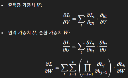
이 과정에서 나타나는 체인 곱 연산이 gradient vanishing의 근본 원인

💡 고유 통찰 (Insights)

구분	통찰
🔁 순환성	과거 정보를 유지함으로써 문맥 보존 가능
🔃 파라미터 공유	파라미터 수 감소 및 시계열 일반화 학습 유도
🧮 수학적 연산	BPTT는 시간적 unfold를 기반으로 한 복합 연쇄 미분
⚠️ 한계	긴 시퀀스일수록 gradient가 사라짐 (Vanishing)
🧠 확장 구조	양방향 RNN, 다층 RNN, 인코더-디코더 등으로 다양한 과제 대응

🧾 결론

이번 강의는 단순히 RNN 구조를 소개하는 데 그치지 않고, 수식 기반의 학습 구조(BPTT), 시간 축의 파라미터 흐름, 다양한 응용 구조, 그리고 Gradient Vanishing 문제의 원인까지 심도 있게 설명하며, 다음 강의의 LSTM 소개로 자연스럽게 연결됩니다.

00:00:00 In the previous lectures, we learned the mechanism of convolutional neural networks and some advanced CN models for image processing. In this lecture, we learn how the recurrent neural networks work for signal processing. Then let's first see the basic structure of the RNN. This illustration represents the basic real networks. So in the model you can put the input to the hidden layer and then the hidden layer output the estimated labels like this. In the basic RNN structure you can see the recurrence to

00:00:53 pass which can update their weights itself. That means in the RNN architecture the weights of hidden layers are updated according to not only the input but also the previous hidden layers. So we can represent the concept of RNN with this equation. So you can see that the value of a hidden layer in the current step T are determined by the interaction between the input and the value of previous hidden layers. Please note that there is also time step t for the input. Because of the characteristics of RNA, we can process

00:01:53 sequence input X with this recurrent formula. One of the important concept in the RNA is the same function and the same set of parameter are used at every time step. So in this architecture there are three different set of parameters. First there is weights between the input and hidden layer. Also there is the weights between the hidden layer and outputs. Finally there are some weights between the current hidden layers and the previous hidden layers. These three different set of parameters are iteratively used at every

00:02:55 time step. Generally as the interaction function weighted the sum of the previous hidden layer and the current input with tangent h activation function in RNN structure and the output will be determined based on the hidden layer and the weights between the hidden layer and the output layer. And according to the task of RNN, we can set the different activation function for the output. Now let's unfold the recurrent formula and the recurrent structures for better understanding. Now you can see the unfolded RNN

00:03:52 structures according to every time step t. In the time step t, the hidden layer will be determined based on the current input x and the previous hidden layer according to the this formula. And the output could be induced based on the current hidden layer and the weights between the hidden layer and the output. The updated hidden layer will be fed to the next step hidden layer and then the next hidden layer will be updated based on the previous hidden layer and the next step input. As mentioned before in the

00:04:56 recurrent process every waste will be reused at every time steps. So in this architecture we have three different set of parameters like this and we use the same weight value for each set of parameters. at every time step. So that is the forward propagation in RNN. After the for propagation, we can measure the difference that means loss between the estimated output and the real output for every time step like this. And we can measure the total loss by accumulate the loss of every time steps like

00:06:06 this. Now let's see the back propagations of RNN. After we compute the total errors of our RNA model, the error will be also passed to the previous layers through entire sequence to compute gradient and then update every weights of the RNN in the hidden layer because of the recurrent pass the error also passed to the previous hidden layer. So it is coded as back propagation through time. Now let's see the details of the forward and backward propagation in RNN with mathematics. So these are summarized for the

00:07:11 propagations in RNN. So I represent the different set of parameter with V, W and U. So the current hidden layer will be determined based on the weighted sum of the previous hidden layer and input X with activation function tangent H. And the output will be determined with the weighted hidden layer. And we measure the difference between the estimated output and the real output at every time step. Moreover, we sum the errors at every time step to measure the total loss. So these are the four propagation

00:08:17 in RNS as shown before. Now let's see the back propagation in RNN. You may remember that in the neuron network training we will measure the gradient to update every weight parameters and we can use the partition dates to measure the gradient for each weight parameter like this. So now let's measure the gradient of error with respect to the parameter U and parameter W respectively. Please note that the gradient of error respected to B is the same as the conventional neural network training steps. So in

00:09:17 this lecture we only consider these two cases. So the gradient two of error respect to u is equal to the summation of the gradient of errors at every time steps respect to the u. Right? You can just simply solve these equations with back propagation. By using the chain rule, we can divide this term to these two elements. You can simply see that these two equation are equal. According to the distance, the second element will be calculated as this one and the first element will be easily calculated according to the error

00:10:25 function. You may remember that we can use the mean square error loss function for regression and cross center field loss for classification. So according to the error function we can simply measure distance and according to the this equation we can solve the second element with this one. Just simply think that the back propagation on here and here are same as the conventional neuron nets. The main part of the back propagation in RNN is the recurrent part. So let's see how we can measure the gradient of error at every time step

00:11:26 t respect to the w. We can also use the channel to divide this term into this one. So you can also see that these terms are same. So you can simply follow here by using these terms. So the first so the first element is same as the previous one. So we can simply measure the gradient when we have the error function. Now let's see the second term. So actually these two terms are came from here right. So, so when we see the this one only the hidden layer are related to the W. So we can divide this term according to the hidden

00:12:55 layer like this. So we can also simply measure the second term. Now let's see the last one. Actually this part is the main back propagation steps in RNN. To measure the gradient, we need to perform the partition der of this terms according to the W. Right? So you may know that this term is not related to the W. So you can remove this term and you can only consider this one. You may know that if the H is not related to the W, we can simply calculate it the partition debate like this one. However, the main problem

00:14:01 is this H is also have the W, right? This is becomes the more previous layer like this. So this H is also contain the W parameter. So this is becomes the product derivate for two different function related to the same parameter. So you can remember that we can solve the problem with product rule of the der like this. So we need to go back through the time until the first time step. So we can represent this term to this one. So these two equation represent the product rule of the particial der of

00:15:37 h. So this one is came from the derivate of the activation function and actually we need to measure this one and as mentioned before we don't care this term and we only care this one and as mentioned before with the product to rule of the der like Yes. We first have the H with this one and then we also get the additional gradient for this one because this H also contain the W, right? So this term will be recursively added for the previous layers. So we need to this summation equation for the average time

00:16:56 step. So this term indicates these two pumps and this indicate the rest. So according to the this kind of process we can measure the gradient of the error respect to the each weight and by using the gradient we can update every weights during the back propagation. There are different types of RNN according to their task. So the first one is basic feed for the neuron networks as shown before which consist of input feed layer and the output compared to the basic neural network RNN can have different type

00:17:57 according to the task. So the first one is one too many and in the architecture we only have a single input while we have multiple outputs at the different time steps. The most well-known application in this type is image captioning. So for example, if we put a single image to the RNA model, the RNN will generate some sentence to represent the input. In the other case, we can put the sequence data to RNA and then get the single output. For this case, you can image sentimental classification in the application. If

00:19:00 you put the sentence to RNN, the RNN will classify your sentiment. For other applications like machine translations, you can put the sentence to the RNN and then get the another sentence from RNN. You can image that you put the Korean sentence to the RNN then the RNN realize your sentence and then change it the sentence to English. So this parts of RNN work for encoding your input and the rest part of RNN will work for decoding your input. Please note that in this case the input and outputs are asynchronized.

00:20:09 For example, in machine translation, the size of input and output could be different. In the other types of RNM, we can construct the synchronized input and output. In the other case of RNN, we can construct our RNA models for synchronized input and output. For example, in frame level video classification. When you put a single frame of video that means image you can directly get some result from your RNN. In some case we can also stack multiple recurrent hidden layer like this. Moreover, in some case we can construct

00:21:22 birectional RNN. Actually in many sequence data both the forward and backward information flow are important. However, in the previous RNA model, only the forward flow are considered to process the sigma. To solve the limitation in the biirectional RNA, there are two different flows. The first one is forward flow and the next one is the backward information flow. and the output will be determined based on the forward and backward flow together in the birectional RNN architecture. So now let's summarize the

00:22:23 RNN with their gradient flow. This image illustrate the forward propagations in the hidden layer. So we have the input at the time point t and also have the hidden layers at the previous time. And we have the tangent h function for the activation. And now we can measure the value of the current H based on the weighted sum of the previous layer and the input. When we check the back propagations in RNN, we saw many multiplication of W when we go through the previous time step. You may remember these terms in the back

00:23:31 propagation step right. So during this step we have the multipation of the W for every time step. So when we perform the back propagation or times we need to multiply many w. So just simply think if we multiply a smaller value than one many times then the value becomes zero. Right? So when we perform the back propagation through time there is a vanishing gradient problem at the very early time step that means in the basic RNN structure it is very hard to run a longterm dependency. So in the next lecture we will learn the

00:24:46 long short-term memory model which is the advanced RNN model to solve the gradient vanishing problem and also see the several applications by using RNN. So please let me know if you have any question. Thank you.

Summary

This lecture delves into the fundamentals of Recurrent Neural Networks (RNNs) and their application in signal processing, contrasting them with Convolutional Neural Networks (CNNs) previously discussed for image processing. The core architecture of RNNs is introduced, emphasizing that hidden layer weights are updated based both on the current input and the previous hidden layer’s output, enabling the processing of sequential data over time steps. The lecture explains the forward pass mechanics, including the recurrent nature of parameter usage, activation functions, and output generation.

Further, the session elaborates on unfolding the RNN structure in time to clarify how the recurrent computations propagate forward across steps. It then covers backpropagation through time (BPTT), focusing on how error gradients are calculated and propagated backward through every time step to update weights. The mathematical formulation for forward and backward passes, involving parameter sets (V, W, U), the chain rule, and gradient calculations, are explained in detail, highlighting the recursive nature of gradient updates due to parameter reuse across time.

The lecture introduces different RNN architectures tailored to various tasks, including one-to-many (e.g., image captioning), many-to-one (e.g., sentiment classification), many-to-many with asynchronous input and output sizes (e.g., machine translation), and synchronized input-output models (e.g., frame-level video classification). Advanced structures like stacked RNN layers and bidirectional RNNs are also discussed, the latter addressing the limitation of unidirectional information flow by incorporating backward passes for better context understanding.

Finally, the lecture highlights a crucial challenge: the vanishing gradient problem during backpropagation through long sequences, making it difficult for basic RNNs to capture long-term dependencies. This sets the stage for the next lecture on Long Short-Term Memory (LSTM) networks, which are designed to overcome this issue.

Highlights
🔄 RNNs update hidden layer weights based on current input and previous hidden states, enabling sequential data processing.
📊 Forward propagation in RNN reuses the same set of parameters at each time step, maintaining model consistency.
🔙 Backpropagation through time (BPTT) calculates gradients recursively across all time steps to update RNN weights effectively.
🧮 Detailed mathematical insights show how gradients are computed using the chain and product rules in RNN training.
📝 Different RNN architectures fit different tasks: one-to-many, many-to-one, many-to-many (asynchronous and synchronous).
🔄 Bidirectional RNNs improve performance by integrating forward and backward information flows for sequence processing.
⚠️ Basic RNNs suffer from vanishing gradient problems during BPTT, limiting their ability to learn long-term dependencies.
Key Insights
🔁 Recurrence enables temporal context retention: Unlike feedforward networks, RNNs incorporate feedback loops by passing hidden states from one time step to the next. This feedback mechanism allows models to remember information from previous inputs, making RNNs well-suited for sequential data such as signals, text, or time series.
🔧 Parameter sharing across time steps: RNNs use a fixed set of parameters (weights) repeatedly at every time step, which reduces the number of parameters and forces the network to generalize temporal patterns rather than memorize specific instances at each position, enhancing training efficiency and robustness.
🧮 Backward propagation through time (BPTT) is essential but complex: BPTT extends traditional backpropagation by unfolding the network along the temporal dimension. This unfolding results in recursive computations of gradients that involve chain and product rules, which can be mathematically intensive but are critical for aligning model predictions to true sequences.
🔄 Bidirectional execution captures context better: Standard RNNs consider past information only, but bidirectional RNNs process data in both forward and backward time directions, allowing the model to access context from both preceding and succeeding parts of sequence data, improving accuracy in many NLP and signal processing tasks.
🧠 Task-specific RNN architectures optimize performance: The diversity of tasks — from producing multiple outputs from a single input (one-to-many) to transforming sequences of different lengths (many-to-many) — requires different RNN variants. This customization emphasizes RNN versatility across domains like image captioning, sentiment analysis, and machine translation.
⚠️ Vanishing gradient problem inhibits long-term dependency learning: Due to repeated multiplication of small weight values during backpropagation, gradients can diminish exponentially, making it difficult for basic RNNs to learn dependencies over long sequences. This insight motivates the need for more sophisticated architectures like LSTMs or GRUs.
🔍 Mathematical rigor underpins RNN training: Understanding RNNs requires grasping how errors propagate through time, how weights influence hidden states recursively, and how activation functions and loss functions interplay. Mastery of these concepts enables effective model design, training adjustments, and troubleshooting.

This lecture provides a comprehensive foundation on RNN theory, forward/backward propagation mechanics, various architectural adaptations, and the challenges faced, perfectly setting the stage for advanced recurrent architectures specialized in overcoming fundamental RNN limitations.

9강 - LSTM

📌 핵심 요약: Long Short-Term Memory (LSTM)

1. 배경: RNN의 Gradient Vanishing 문제

문제점: 기본 RNN은 긴 시퀀스를 처리할 때 기울기 소실(Vanishing Gradient) 문제로 인해 장기적인 의존 관계(long-term dependency)를 학습하는 데 한계가 있음.
- 예: 시간 t 시점의 은닉 상태 h_0에 대해 기울기를 계산할 경우 W에 대한 다수의 곱이 필요 → 기울기 폭발 혹은 소실.
- 참고: Bengio et al. (1994), Pascanu et al. (ICML 2013)

🔍 LSTM 구조: 세 가지 게이트와 셀 상태

LSTM은 Hochreiter & Schmidhuber (1997)에 의해 제안된 구조로, 세 가지 게이트와 셀 상태(Cell state)를 도입하여 RNN의 한계를 해결함.

1. 🧠 셀 상태 c_t

장기적인 정보를 저장하는 경로로서, 기울기 흐름을 방해받지 않고 전달할 수 있는 핵심 구조.

2. 🔑 게이트 구성 요소

각 게이트는 모두 시그모이드 함수와 탠젠트 하이퍼볼릭(tanh)를 조합하여 작동하며, 0~1 사이 값을 출력함.

게이트 종류	수식적 의미	역할 설명
Forget Gate f_t		과거 정보를 얼마나 잊을지 결정
Input Gate i_t, Candidate c^~_t		현재 입력으로부터 얼마나 저장할지 판단
Output Gate o_t		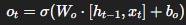최종 출력을 얼마나 드러낼지 결정

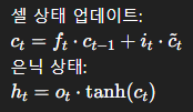
⚙️ Gradient Flow in LSTM

LSTM의 셀 상태 c_t 경로는 기울기 소실 없이 정보가 전달될 수 있도록 설계됨 → 기울기의 단절 없는 흐름(Uninterrupted gradient flow) 보장

🎯 응용 사례

1. 시퀀스 생성 (RNN 기반 응용)

소설 작성, 교과서 작성, C 코드 생성 등 다양한 텍스트 생성 작업에 활용됨

2. 이미지 캡셔닝 (Image Captioning)

CNN → RNN 조합 구조
- CNN이 이미지 특징을 추출하고, RNN (또는 LSTM)이 텍스트로 변환
- Karpathy et al. (CVPR 2015)

3. 어텐션 기반 이미지 캡셔닝

Attention Mechanism을 도입한 구조 (Xu et al., ICML 2015)
- 입력 이미지의 특정 위치에 주의를 집중하여 설명 생성

4. 시각적 질문 응답 (Visual Question Answering)

이미지와 질문을 받아 답변을 생성
- Agrawal et al. (ICCV 2015), Zhu et al. (CVPR 2016)

✅ 정리된 통찰

LSTM은 RNN의 구조적 한계를 극복하고 장기 의존성 학습, 안정적인 기울기 전달, 다양한 시퀀스 기반 문제 해결을 가능하게 하는 중요한 딥러닝 모델임
Attention과 결합될 경우, 더욱 복잡한 시각-언어 융합 문제에 대해 높은 성능을 발휘함

📌 LSTM 강의 대본 요약 (중복 없는 핵심 중심)

1. 🔁 RNN 복습과 한계

RNN은 시퀀스 입력을 다룰 수 있는 구조이며, 시점별로 입력과 이전 은닉 상태를 통해 현재 은닉 상태를 갱신.
손실은 시점별로 계산되며, 역전파 시 전체 시퀀스를 따라 Backpropagation Through Time (BPTT) 적용.
다양한 구조 (one-to-many, many-to-one, many-to-many async/sync) 및 bidirectional, stacked RNN 설명.
하지만 vanishing gradient 문제로 인해 긴 의존성을 학습하는 데 실패 → 해결책: LSTM

2. 🧠 LSTM 구조와 작동 방식의 직관적 해석

LSTM의 핵심은 셀 상태(cell state)를 통한 장기 정보 전달이며, 세 개의 게이트가 이를 제어한다:

🔒 Forget Gate

입력: 이전 은닉 상태, 현재 입력
연산: 시그모이드 → 0~1 사이의 스칼라 값 생성
역할: 이전 셀 상태를 얼마나 지울지 결정
직관: 0이면 완전 삭제, 1이면 유지

📝 Input Gate

두 연산 분리:
- 시그모이드 → 어느 정보를 저장할지 결정
- tanh → 새로운 후보 값 생성
역할: 현재 시점의 입력 정보를 셀 상태에 얼마나 저장할지 조절
기존 RNN의 forward 연산에 "가중치 필터"가 추가된 구조

📤 Output Gate

셀 정보를 tanh로 변환한 후 시그모이드와 곱함
역할: 셀 상태에서 얼마나 정보를 꺼내 은닉 상태로 보낼지 결정
직관: 출력을 조절하는 "밸브"

✅ 요약:

셀 상태는 연속적으로 정보를 보존하는 경로이며, 세 게이트는 기억, 저장, 꺼냄을 각각 담당
LSTM은 각 게이트의 조합으로 셀 정보를 정제하며, 복잡한 시퀀스에서도 정보 손실 없이 흐름을 유지함

3. 🧮 Vanishing Gradient 문제 해결의 직관

RNN: 반복되는 W × W × W … 연산 → 기울기 소실
LSTM: 셀 간에는 직접적인 weight 곱이 없음 → 기울기가 셀 상태 경로를 따라 방해 없이 흐름
각 게이트의 내부 가중치는 셀 내부에서만 작용하며 기울기 흐름의 병목을 방지

🔑 LSTM은 “기울기 고속도로”를 만들어 멀리 있는 정보도 손실 없이 전달 가능하게 만듦

4. 📚 실세계 응용 사례

📖 1) 소설 생성 (Novel Writing)

RNN 기반 생성 모델이 학습 초반에는 무의미한 문장을 생성하다가 학습이 진행되면서 점차 자연스러운 언어 생성
실제 문법적으로 오류 있는 텍스트도 있음 → 향후 강화 가능성 강조

📘 2) 교과서 생성

실제 교재를 학습한 뒤 유사한 스타일의 문장과 수식을 생성함
초창기에는 오답 및 불완전한 표현이 많지만, 형식적으로 근접한 결과 가능

🧑‍💻 3) 코드 생성

RNN이 C 언어 코드를 자동 생성 → 실제 실행 가능
반복적인 구조나 패턴을 학습해 구조적인 코드 문법 생성 가능

🖼️ 4) 이미지 캡셔닝 (Image Captioning)

구조: CNN → RNN
- CNN: 이미지 임베딩 추출
- RNN: 텍스트 시퀀스 생성
성능: 전반적으로 우수하지만, 문맥 오해 예시 존재
- 예: iPhone을 mouse로 착각한 결과 등

🎯 5) 시각 질문 응답 (Visual Question Answering)

CNN이 이미지를 처리하고, RNN이 질문을 분석 → 두 정보 융합으로 답변 생성
텍스트-비전 융합 작업의 대표적 사례로 소개됨

✅ 정리된 통찰

항목	핵심 내용
LSTM의 핵심	셀 상태 + 세 게이트 구조로 장기 의존성 학습 가능
기울기 흐름	셀 상태를 통한 uninterrupted gradient → vanishing gradient 방지
게이트 역할	Forget: 기억 제거 / Input: 정보 저장 / Output: 출력 제어
응용 확장성	문장 생성, 코드 작성, 이미지 캡셔닝, VQA 등 다양한 실세계 문제 해결 가능
설계 직관	게이트별로 분리된 함수와 경로가 학습 안정성과 해석 가능성을 높임

📘 LSTM 강의 요약 (강의 자료/대본 미중복 확장 중심)

🔧 기술 개념 확장 및 세밀한 직관

🧠 셀 상태(Cell State)의 역할은 단순한 정보 저장이 아니다

LSTM의 핵심은 은닉 상태(hidden state)와는 별도로 유지되는 셀 상태(cell state)임
이는 단순히 데이터를 보존하는 버퍼가 아니라, 시간 축을 따라 오차(gradient)가 손실 없이 흐를 수 있도록 설계된 경로
즉, 셀 상태는 기울기 보존 경로로서 작용하며, 오차 역전파(backpropagation)를 도와 장기 의존성(long-term dependency)을 학습 가능하게 함

⚙️ 게이트의 수학적 의미는 “경로 선택 함수”

세 게이트는 모두 시그모이드(σ) 함수를 사용하여 0~1 사이의 값을 생성함
이 값은 곧 “해당 정보를 얼만큼 반영할지” 결정하는 가중치 역할
- Forget Gate → 과거 정보 제거 여부
- Input Gate → 새로운 정보 반영 정도
- Output Gate → 셀 상태 중 어느 정도를 은닉 상태로 보낼지 결정
따라서 게이트는 단순한 "스위치"가 아닌, 정보 통과량을 조절하는 필터

🔁 Backpropagation 흐름과 게이트의 배치

기본 RNN에서는 시점 간 weight W 곱이 누적 → 기울기 소실 발생
LSTM은 셀 간 weight 곱이 없음 → 기울기가 직접 흐름
게이트 내부 연산에만 weight 곱이 존재하여, 기울기 흐름을 차단하지 않도록 구조화됨
이를 통해 가중치 경로는 학습의 유연성을 제공하되, 정보 경로는 안정성을 제공

📐 구조 차이 vs 성능 차이

RNN과 LSTM 모두 시퀀스를 다루지만, 구조 차이로 인해 처리 가능 시간 범위가 극단적으로 다름
- Vanilla RNN은 보통 5~10 step 정도의 정보만 유의미하게 학습 가능
- LSTM은 수백 step 길이의 의존성도 유지 가능

🧪 실제 응용에서의 미묘한 관찰들

📖 자연어 생성 (Text Generation)

AI가 소설, 교과서, 코드 등을 생성할 수 있음은 단순한 언어 패턴 학습에 기반
하지만 문맥 유지(context coherence)는 여전히 어려운 과제이며, 이는 cell state를 어떻게 관리하느냐에 달려 있음
예: 등장인물의 이름을 초반에 보고, 수천 토큰 뒤에서 다시 언급하는 능력은 LSTM의 대표적인 장점

📷 이미지 캡셔닝에서 CNN+LSTM 구조의 실제 흐름

CNN이 추출한 feature map은 평균 풀링이나 FC layer를 통해 고정 길이 벡터로 변환됨
이 벡터는 LSTM의 첫 번째 시점(hidden state 초기화)에 사용되어, 이미지를 “문맥”으로서 이해하게 함
이후 RNN은 단어를 시퀀셜하게 생성 → 이전 단어를 현재 단어 예측에 반영

❓ VQA는 단순한 Q&A가 아니다

시각적 질문응답(VQA)은 멀티모달 융합의 대표적 사례
CNN → 시각적 특징 추출
RNN → 질의 문장의 시퀀스 이해
Attention → 질문의 초점이 되는 이미지 영역 강조
이처럼 VQA는 LSTM이 문장을 이해하는 능력과 시각적 컨텍스트를 조정하는 메커니즘이 합쳐져야 가능

📌 주요 차별화 포인트 정리

항목	기존 내용	이번 요약에서 보완한 내용
셀 상태 개념	정보 저장의 경로	기울기 보존 통로로서의 기능 강조
게이트 직관	시그모이드 기반 필터링	수학적으로 ‘정보 통과량 제어 장치’로 해석
기울기 흐름	소멸 방지로 요약	게이트 내부 배치와 곱 연산 위치의 차이까지 분석
텍스트 생성	소설, 교재, 코드 등 가능	문맥 유지와 장기 의존성 학습 예시 추가
이미지 캡셔닝	CNN+RNN 구조	첫 hidden state 초기화 방식 및 attention 적용
VQA	멀티모달 융합	문장-이미지 동시 해석 구조와 attention 동작 설명

✅ 결론

이 강의는 LSTM의 구조적 강점을 기술적으로 정교하게 해석하는 동시에, 실제 문제에서의 시퀀스 모델링 응용 능력을 구체적으로 보여줍니다. 단순히 “기울기 소멸을 해결한다”는 선언에 그치지 않고, 기울기 흐름의 세부 구조와 그에 따른 학습 안정성을 이해해야 LSTM의 진정한 강점을 실감할 수 있습니다.

00:00:01 In the previous lecture, we learned recurrent neural networks. In this lecture, we will learn the advanced recurrent neural network methods which is ced as RS10 long short-term memory. Let's first remind the previous lecture. In the lecture, we first learned the recurrent structure of RNN. With the recurrent structure, the hidden layer is determined based on the previous hidden layer and the current input layer. Because of the recurrent formula, the RNA can take the sequence input like this. We also saw the forward propagation in

00:00:51 RNN throughout the entire sequence to compute loss at every time stamp in the backward propagation in RNN. We saw that the loss is passed backward throughout the entire sequence to compute gradient. So we can call the process as back propagation through time. We also checked different types of RNN. So we saw one to many types for image captioning and many to one type for semantic classification. We also saw the many to many types which have the asynchronized input and output for machine translation.

00:01:43 Finally, we also saw the different many to many types which have synchronized the input and output for frame level video classification. We also learned that we can stack multiple hidden layer in RNN and we can also stack the birectional RNN. Finally, we run that the RNN has the vanishing gradient problem. So it is hard to run a long-term dependency to solve the problem of vanilla RNA. The LSTM model was proposed. So this is illustration of the inside of heat layer in LSTM. There are three different gate. So

00:02:35 we will see them one by one. Before that we first check the concept of the cell instant. Just think the cell is the strategy to save the information of the hidden layer. So we can save the hidden information to cell or we can restore the hidden informations from cell. The first gate determines how much information from the previous hidden layer will be stored to cell. You can see that the gate takes two inputs. The previous hidden layer and the current input. You can also see the gate has a sigmoid function.

00:03:33 The output of the sigmoid function is a value between zero and one. So in summary, the function takes two input, the previous hidden layer and current input and then the information is fed to the sigmoid function to generate a value between zero and one. In the first gate, the value will be multiplied to the previous cell. That means the value of the function will perform as a weight of the previous cell. And as I mentioned before, the value of the function will be less than one because of the sigmoid function.

00:04:32 So because of that the function will perform to reduce the cell information. This is why the first cell is coded as the forget gate. So in the forget gate the rest determine whether to erase cell. You can simply think that if the value of the function is zero then we don't take any information from the previous cell and if the value of the function is one then we fully takes the previous cell information. Now let's see the second gate. So this is the structure of the second gate. You can see the two different

00:05:31 function. The sigmoid function and tangent h function. The sigmoid function also performed as the width generation. And you may see that the tangent h function in the for propagation in RNA. So this process is the same as the for propagation in the vanilla RNA. So you may remember that in the for propagation in RNN the hidden layer takes two input the previous hidden layer and the current input and then based on the tangent edge we can determine the current hidden layer. Right? In the second gate in RSTM

00:06:30 we additionally have a weight function. So in the second gate in RSTM we will perform the weighted forward propagation and then save the information to the cell. So the second gate is recorded as input gate. The gate determines how much information generated by the for propagation in RNN to be saved in cell. So based on the forget gate we will get the information from the previous cell and based on the input gate we will get the information from the previous hidden layer and current input. Now let's see the last gate in

00:07:29 LSTM. You can also see the sigmoid function in the last gate and you may know that the gate will perform as weight generation. So it will generate a value between zero and one same as the previous gate. You can also see the tangent h function in the pipeline. The tangent edge function takes information from cell and pass the information to the next hidden layer and the sigmoid determines the weight of the information. As the cell information is restored and then passed to the hidden layer, this gate is ced as output gate.

00:08:28 The gate determines how much information from the cell should be revealed. So this is overall process of the arm. So in the forget gate we can decide whether to receive information from the previous cell or not. And in the input gate we will get the weighted information from the current input and the previous hidden layer. And in the upper gate we will get the weighted information from the cell and then passed to the information to the current hidden layer. Now let's think that how the RTM reduced the gradient vanishing

00:09:19 problem in vanilla RN. Please remind that the multiple multiplication of W in RNN caused the gradient vanishing problem in back propagation. Now let's check the gradient flow in RSTM. In the RSTM the gradient to are passed through the cell instead of the hidden layer. You can see that there is no weight multiplication between cell even though there are some weights in inside of each cell. So in the STM the gradient flow is not interrupted between cells and each weight will be updated in the inside of

00:10:20 the cell respectively. You can simply think that the weights become the obstacle of the gradient glow in RNN. But in RSM they put the weight in the inside of the cell so that the gradient will be passed through the cell without any obstruction. Now let's see several examples and applications of RNA. The first application is Nobel writing. You may heard that some AI robots wrote Nobells. The robots is based on RNN models. You can see that in the early training step, the RNN generated incomprehensible sentence like

00:11:17 this. However, after more and more training, the RNN can generate some readable sentence like this. So based on the RNA models, we can make some AI robot to write Nobels. We can also write some text books like this. The RNN is trained by the real text book and then the RNN generates some fake textbook like this. Actually this equation and the sentence will be wrong. But anyway Darin makes some plausible sentence or equations for textbook. If we keep training the RNN, then someday we could make a real

00:12:23 textbook. The RNN can make the AI to generate their programs itself. So this code is generated by the RNN and and surprisingly this code could be run in C program. The next two application is image captioning. The goal of the image captioning is generate some sentence which can describe the images. So in the first part based on the CNN we can generate the embedded vector feature vector which contains some special information of the image. Now in the next part we construct the RNA model to train the sentence related to

00:13:21 the image to understand the immediate features in RNN. The hidden layers of RNN takes the additional input from the embedded feature vectors of CNN. Based on the additional input, the RNN can generate some sentence related to the images. These are the results of the image captioning. So you can see that there are many successful captioning result related to the input image. Of course, there are still some errors in the captioning according to the performance of the CNN and RNA models. For example, in this

00:14:14 case, the model realized that the iPhone as mouse because there is laptop on the table. If we construct the CNN model with attention mechanism, then we can also perform this kinds of work. With the attention module, the CNN can understand the important part of the image to generate this caption. Visual question and answering is one of the most widely studied application for image and sentence. The main goal of BQA is generating an answer based on the image and the sentence of the question. So based on the CNN we can understand

00:15:11 the features of image and based on the RNN we can understand the questions. So based on the CNN and IN hybrid model we can generate some answers related to the image and the questions. So in this lecture we learned that how the arm works and how to solve the problems of vanilla RNN. Moreover we saw that how the stem and RNN models are used for real applications. Please contact me by this email if you have any question. Thank you.

Summary

This lecture builds upon the foundational concepts of recurrent neural networks (RNNs) by introducing advanced recurrent neural network methods, specifically Long Short-Term Memory (LSTM) networks. The lecture revisits the RNN structure which processes sequential data by maintaining hidden states influenced by both current inputs and previous hidden states. It reviews various RNN types such as one-to-many, many-to-one, and many-to-many architectures and highlights challenges like the vanishing gradient problem prevalent in vanilla RNNs. To address this, LSTMs were proposed with a unique cell state mechanism regulated by three gates (forget gate, input gate, and output gate) to selectively store, update, and propagate information over long sequences without losing gradients. The lecture delves deeply into each gate’s operations, illustrating how these gates control the flow of information and maintain gradient stability. Finally, practical applications of RNNs and LSTMs are introduced, including AI-based novel writing, textbook generation, program code creation, image captioning, and visual question answering, demonstrating the versatility and progress of these advanced models in real-world scenarios.

Highlights
🔄 Recap of vanilla RNN structure and types (one-to-many, many-to-one, many-to-many).
🚫 Explanation of the vanishing gradient problem in vanilla RNNs.
🔐 Detailed breakdown of LSTM gates: forget gate, input gate, and output gate.
📈 Explanation of how LSTMs maintain gradient flow via cell state, avoiding vanishing gradients.
🤖 Applications: AI-generated novels, textbooks, and executable computer code.
🖼️ Image captioning using CNN-RNN hybrid models for feature extraction and sentence generation.
❓ Visual question answering combining CNNs for images and RNNs for language understanding.
Key Insights

🔄 Sequential processing with RNNs demands handling long-term dependencies:
Vanilla RNNs process sequences by passing hidden states through multiple time steps. However, their recurrent weight multiplication often causes gradients to vanish or explode during backpropagation, limiting their ability to learn long-term dependencies in sequence data.

🔐 LSTM cells incorporate gates to regulate information flow and overcome vanishing gradients:
The invention of forget, input, and output gates within LSTM cells actively manages what information to retain, update, or output. This gating mechanism enables the network to selectively preserve crucial information across long time steps, greatly improving learning over sequences.

🔄 The cell state in LSTM enables uninterrupted gradient flow during backpropagation:
Unlike vanilla RNNs where gradients are repeatedly multiplied by weights causing decay, LSTM cell states allow gradient flow with minimal interference, as weights reside inside gates rather than directly on recurrent connections between cells. This prevents gradient vanishing and enables effective long-range learning.

🤖 RNNs and LSTMs can generate complex sequential outputs such as text or code:
Training with large datasets, these models can produce increasingly coherent and viable sentences, code snippets, or even entire documents by learning statistical patterns in sequences. While initial outputs may be nonsensical, continuous training improves fluency and relevance.

🖼️ Combining CNNs and RNNs enables image-to-text applications like image captioning:
CNNs extract image feature vectors that are fed into RNNs to generate descriptive sentences. Although errors exist (e.g., mislabeling objects), the use of attention mechanisms enhances accuracy by focusing on relevant parts of images, improving caption quality.

❓ Visual Question Answering (VQA) leverages CNNs for image understanding and RNNs for question interpretation:
By integrating visual and textual data, the hybrid model can produce answers that relate to both the content of an image and the semantics of a question. This approach highlights the synergistic capability of multi-modal deep learning frameworks.

🚀 Advanced RNN architectures like LSTMs have revolutionized sequence modeling tasks across domains:
With their ability to manage long-term context and avoid gradient problems, these models underpin many state-of-the-art solutions in natural language processing, computer vision, and AI-generated content, marking a substantial evolution from vanilla RNNs.

This lecture thoroughly illuminated the significance of LSTM networks in advancing recurrent neural network capabilities and showcased diverse impactful applications, underscoring their importance in modern AI research and deployment.

저작자표시 비영리 (새창열림)

'인공지능 > 공부' 카테고리의 다른 글

딥러닝 총 정리 (2)	2025.07.04
딥러닝 공부하기 3 (4)	2025.07.03
딥러닝 공부하기 1 (1)	2025.07.01
시험 공부 겸 정리하는 곳 - LVLM (0)	2025.04.21
재미있는 인공지능 속 세상 여행 3주차 - Chat GPT의 등장과 비즈니스 환경 변화 (8)	2024.09.18

현재글딥러닝 공부하기 2

NLP, AI, XAI에 관심있는 공대생의 일기장...?

Today :
Yesterday :

« 2026/01 »
일	월	화	수	목	금	토
				1	2	3
4	5	6	7	8	9	10
11	12	13	14	15	16	17
18	19	20	21	22	23	24
25	26	27	28	29	30	31