인공지능/공부

딥러닝 공부하기 1

이게될까 2025. 7. 1. 20:42

728x90

1강 - Deep Learning Intro

🔍 AI, ML, DL의 관계

AI (인공지능): 기계가 인간의 지능을 모방하는 것.
ML (머신러닝): 데이터를 통해 명시적 프로그래밍 없이 학습하는 기술.
DL (딥러닝): 머신러닝의 하위 분야로 신경망(neural network) 기반.

🧠 AI와 DL의 역사

연도	주요 사건
1956	다트머스 회의에서 ‘AI’ 용어 등장 (John McCarthy 등)
1958	퍼셉트론(perceptron) 제안 – 간단한 신경망
1969	퍼셉트론 한계 지적 (XOR 문제 등) → 1차 AI 겨울
1986	다층 퍼셉트론(MLP) 등장
1990s	SVM 등 기타 머신러닝 기술 개발, Deep Blue 등 실용화
1995~2006	딥러닝 개념 부상 → 2차 AI 겨울 이후 재도약
이후	Siri, AlphaGo, 자율주행차 등 딥러닝 기반 AI 활약

⚙️ AI 시스템 구성 요소

입력(Input): 예) 바둑판 상태
과업(Task): 다음 수 결정
출력(Output): 다음 수 후보
수학적으로는 입력 X → 함수 f(X) → 출력 Y의 구조로 이해

🧩 ML과 DL의 차이점

구분	머신러닝 (ML)	딥러닝 (DL)
학습	선행 지식 필요 (피처 엔지니어링 등)	데이터만으로 학습 가능
성능	데이터 많아도 한계 존재	데이터 많을수록 성능 향상 가능
구성	얕은 모델	깊은 신경망 구조 가능

🧠 결론

딥러닝은 더 많은 데이터와 복잡한 모델을 통해 기존 ML보다 뛰어난 성능 달성.
다음 강의에서는 딥러닝을 위한 기초 수학 (선형대수, 확률이론)을 다룰 예정.

00:00:01 in this lecture we will see a brief overview of deam learning let's first talk about the terms of artificial intelligence team learning and machine learning so which one is the largest concept yes then what is the next the next is machine learning and then the dim learning becomes the last one now let's talk about AI what is the ai ai is the simulation of human intelligence processed by machines or computer system then what is the machine learning the machine learning represent techniques that empower the machine to

00:01:00 learn without being splitly programmed then what is the de learning the demm learning is a subset of machine learning based on the neuron networ now let's see the history of AI and dim learning in 1956 John mcy first mentioned the to of AI in a conference two years later the percep which is an algorithm that mimic neurons in the brain was developed but after the year many researchers had realiz the limitations of the perceptron so in the first period of AI most of the AI systems were developed with rule based approach

00:02:01 however many researchers had thought about the rule based AI so there was the first AI winter but during the period some researchers still focus on the perception so they developed the multi-layer perceptron However unfortunately there was still questions about how to train the model so there was the second AI winter in 1990s other machine learning techniques like support Vector machine were developed in the period many machine learning based AI systems like the blue which can play chess game better than

00:02:54 human were proposed in 26 the concept of dim learning was introduced from the year many dim learning method are still being proposed so now we have many te learning based AI systems like Waton CI and arpo until now we first checked the terms of AI machine learning and de learning and then we saw the history of the AI according to the development of the de learning techniques now let's learn more about AI so here we have a box and let's convert this box to an AI system then you first input some data to

00:03:50 the AI system next you have to define the task that the AI system will perform finally you will need desired output according to the test and input now the box is changed to an AI system let's suppose that the AI system is arable then sequence of move in go becomes input and we want the AI system decide the next move to win then the AI will will output the candidate of the next move to win now let's look at the AI system from a mathematical point of view so we can assign some variables to the components of the

00:04:46 system so you can see the input becomes X and output becomes y then we can express the AI as the function of X which generates the Y Accord according to the task so this is AI if you design the function of X according to the task you can make an AI system then how can you make the function you can use the machine learning to make the function of x if you have training input and output data X Prime and Y Prime then you can estimate the function of X so now you can put the estimated function of x to your AI

00:05:43 system if you adopt a better machine learning method the AI system would be smarter by the way actually the machine learning requires an additional input in conventional machine learning to estimate the the function of X we need prior knowledge for learning algorithm however in the te learning we don't need the prior knowledge we only need the training data this is why de learning is so powerful in this day in the traditional machine learning even though you have more data you can't achieve the better

00:06:31 performance however in the demm loing if you have more data you can build deeper and deeper model and then you can achieve better performance from now we have looked at AI machine learning and de learning from multiple perspective in the next lecture we will learn basic mathematics for team learning in linear algebra and property Theory thank you

Summary

This lecture provides an introductory overview of artificial intelligence (AI), machine learning (ML), and deep learning (DL), clarifying their hierarchical relationship and defining key concepts. AI is described as the simulation of human intelligence by machines, while ML refers to techniques that enable machines to learn without explicit programming. Deep learning, a subset of ML, utilizes neural networks to model complex patterns. The lecture also traces the historical development of AI, highlighting major milestones like the introduction of the perceptron, the periods known as AI winters, and the rise of advanced learning methods such as support vector machines and deep learning. Modern AI systems like IBM Watson and AlphaGo exemplify deep learning’s capabilities. Additionally, the lecture explains how AI systems function by mapping inputs (X) to outputs (Y) through mathematical functions, emphasizing that ML helps estimate these functions based on training data. Importantly, deep learning’s significant advantage is its ability to improve performance continuously with increasing data, without requiring prior knowledge, unlike traditional machine learning approaches. The lecture concludes by noting that further exploration of deep learning mathematics, particularly linear algebra, will follow in subsequent lessons.

Highlights
🤖 AI simulates human intelligence in machines, forming the broadest concept.
📊 Machine learning enables machines to learn from data without explicit programming.
🧠 Deep learning is a specialized subset of ML based on neural networks.
🕰️ AI development has faced two notable “AI winters” due to limitations in earlier approaches.
🎮 Modern AI successes include systems like IBM Watson and AlphaGo using deep learning.
🔢 AI models function by mapping inputs (X) to outputs (Y) via learned mathematical functions.
📈 Deep learning’s power lies in improving accuracy with more data, requiring no prior knowledge.
Key Insights
🤖 Hierarchical Structure of AI, ML, and DL: Understanding that AI is the broad field encompassing ML, which itself includes DL, is fundamental. This hierarchy helps clarify how these domains relate, making it easier to grasp why deep learning’s advances have revolutionized AI applications.
🧠 Neural Networks as the Basis for Deep Learning: Deep learning’s use of artificial neural networks allows it to model highly complex data relationships that traditional ML methods struggle with, enabling breakthroughs in image recognition, natural language processing, and more.
🕰️ Historical Context and AI Winters: Recognizing the periods known as the AI winters, caused by too-high expectations and technical limitations, underscores how progress in AI requires both conceptual and computational advancements to sustain momentum.
🔍 Mathematical Representation of AI Systems: Framing AI as a function ( f(X) = Y ) makes clear that AI is essentially about learning the best function to transform input data into desired outputs, where ML (and DL) serve as methods to estimate and improve this function.
📈 Deep Learning’s Advantage with Big Data: Unlike traditional ML, which plateaus even with more data due to reliance on prior knowledge or handcrafted features, deep learning scales with data, building progressively deeper models to enhance performance continuously.
⚙️ The Practical Workflow of AI Systems: From input data provision to defining tasks and obtaining outputs, this process-oriented view emphasizes the application side of AI, making it accessible for practical design and implementation.
📚 Foundational Mathematics is Crucial: The promise of learning linear algebra and probability theory to understand deep learning highlights the importance of strong mathematical foundations for mastering advanced AI techniques.

This comprehensive foundation sets the stage for deeper exploration into AI, machine learning, and especially deep learning in future sessions, equipping learners with both historical perspective and technical understanding.

📘 강의 요약

이 강의는 인공지능(AI), 머신러닝(ML), 딥러닝(DL)의 기본 개념과 이들 간의 계층적 관계를 소개합니다.

AI는 기계가 인간의 지능을 모방하는 광범위한 개념이며,
ML은 명시적인 프로그래밍 없이 데이터를 통해 기계가 스스로 학습하도록 하는 기술입니다.
DL은 신경망에 기반한 ML의 하위 분야로, 복잡한 패턴 인식이 가능합니다.

강의는 퍼셉트론의 등장, AI 겨울, 서포트 벡터 머신(SVM)과 딥러닝의 발전 등을 중심으로 한 AI의 역사를 간략히 정리하며, 현대의 딥러닝 기반 AI 시스템인 Watson, AlphaGo 등을 예시로 소개합니다.

AI 시스템은 입력(X)을 출력(Y)으로 변환하는 수학적 함수로 표현되며, ML은 이 함수를 훈련 데이터(X′, Y′)로 추정합니다.
딥러닝의 핵심 강점은 별도 선행 지식 없이 데이터만으로 성능이 지속적으로 향상된다는 점입니다.

이 강의는 이후 딥러닝을 이해하기 위한 선형대수 및 확률이론 등 기초 수학 강의로 이어질 예정입니다.

📝 주요 포인트 정리

핵심 개념

🤖 AI: 인간 지능의 기계적 시뮬레이션, 가장 상위 개념
📊 ML: 명시적 코드 없이 데이터를 통한 학습
🧠 DL: 신경망 기반의 ML 하위 개념

역사 및 흐름

🕰️ AI 겨울: 기대 대비 성과 부족으로 연구 침체기 발생 (2차례)
🎮 현대 AI: Watson, AlphaGo 등 딥러닝 기반으로 대성공

수학적 이해

🔢 AI 시스템 구조: 입력 X → 함수 f(X) → 출력 Y
🔍 ML/DL은 이 함수를 훈련 데이터를 통해 추정

딥러닝의 강점

📈 데이터 확장성과 성능 향상: 데이터가 많을수록 더 깊은 모델 학습 가능
⚙️ 작동 절차 중심의 시각: 입력-과업-출력 흐름을 중심으로 AI를 이해
📚 수학적 기반의 중요성: 향후 수업에서 다룰 선형대수/확률이론은 필수적 기초

📘 전체 개요 요약

이 강의는 AI, 머신러닝(ML), 딥러닝(DL)의 개념과 관계를 정리하고, AI의 역사, 딥러닝의 구조적 특성, 수학적 표현을 소개하며, 향후 학습에 필요한 수학 기초를 안내합니다.

🧠 핵심 내용 요약

1. AI, ML, DL의 계층적 구조

AI (Artificial Intelligence)
→ 인간 지능을 모방하는 기술 (예: 문제 해결, 판단, 언어 이해 등)
ML (Machine Learning)
→ 데이터로부터 학습하여 규칙을 스스로 추론함
DL (Deep Learning)
→ 신경망(neural network)에 기반한 ML의 하위 분야
→ 복잡한 패턴 인식과 대규모 데이터 처리에 강점

📌 AI ⊃ ML ⊃ DL의 관계

2. AI의 역사

연도	주요 사건
1956	다트머스 회의에서 ‘AI’ 용어 등장
1958	퍼셉트론 (Perceptron) 제안
1969	퍼셉트론의 한계 (XOR 문제) 지적 → 1차 AI 겨울
1986	다층 퍼셉트론 (MLP) 등장
1995	SVM 등 머신러닝 기법 등장
1997	IBM Deep Blue → 체스에서 인간 챔피언 이김
2006	딥러닝 개념 등장
2010~	Siri, Watson, AlphaGo, 자율주행 등 실현

📌 과도한 기대 → 한계 → 침체(AI 겨울) → 기술적 도약의 순환 반복

3. AI 시스템 구조

입력 (Input): 문제를 나타내는 데이터 (예: 바둑판 상태)
과업 (Task): 목표 (예: 다음 수 선택)
출력 (Output): 과업의 결과 (예: 수의 후보)

→ 이를 수학적으로 표현하면:
Y = f(X)
X: 입력, Y: 출력, f: 함수 (학습을 통해 정의됨)

4. ML vs DL의 차이

구분	머신러닝 (ML)	딥러닝 (DL)
특징	특징 추출 필요 (Feature Engineering)	자동 특징 학습 (End-to-End)
입력	학습 알고리즘 + 선지식 필요	선지식 없이 데이터만으로 학습
성능	데이터 증가에 따른 한계 존재	데이터 많을수록 성능 향상 가능
모델 구조	얕은 구조	깊은 신경망 구조 가능

📌 딥러닝은 데이터 확장성과 표현력에서 강력한 장점을 지님

📝 요약 정리

항목	내용
주제	딥러닝의 개념, 역사, 시스템 구조, 수학적 표현
핵심	AI ⊃ ML ⊃ DL 구조, AI의 발전사, f(X)=Y로 표현되는 AI 시스템
차별점	DL은 사전 지식 없이도 데이터로부터 성능 향상 가능
다음 단계	수학 기초(선형대수 및 확률)을 통한 딥러닝 심화 학습

2강 - 딥러닝 수학

📘 전체 구조 요약

파트	내용
1부	선형대수 기초 (Linear Algebra Basics)
2부	확률 및 정보이론 (Probability and Information Theory)

🔢 1부: 선형대수 기초

📌 주요 개념 정리

개념	설명
스칼라 (Scalar)	단일 숫자
벡터 (Vector)	숫자의 배열 (1차원)
행렬 (Matrix)	2차원 숫자 배열
텐서 (Tensor)	n차원 숫자 배열

✏️ 기본 연산

행렬 덧셈 및 행렬 곱셈 (dot product)
- 분배법칙, 결합법칙은 성립
- 교환법칙은 성립하지 않음

🔁 주요 연산

연산	설명
전치 (Transpose)	행과 열을 뒤바꿈
항등행렬 (Identity)	곱해도 원래 행렬 유지
역행렬 (Inverse)	곱해서 항등행렬이 되는 행렬
트레이스 (Trace)	대각선 원소의 합

📐 벡터 및 행렬 속성

개념	설명
노름 (Norm)	벡터의 크기 측정 (L1, L2 등)
선형 독립 (Linear Independence)	벡터들이 서로 종속되지 않음
랭크 (Rank)	선형 독립인 열의 최대 개수
단위벡터, 대각행렬, 대칭행렬 등도 소개됨

🎲 2부: 확률 및 정보이론

📊 확률 기초 개념

개념	설명
확률변수 (Random Variable)	예: 동전 던지기, 주사위 등
이산 분포 (PMF)	정수값 변수에 대한 확률 분포
연속 분포 (PDF)	실수값 변수에 대한 확률 밀도

🔗 복합 확률

결합 확률 (Joint Probability): 여러 변수 동시 분포
주변 확률 (Marginal Probability): 부분 변수에 대한 분포
조건부 확률 (Conditional Probability): 조건 하에서의 확률
체인 룰 (Chain Rule): 결합 확률을 조건부 확률로 분해

🤝 독립성

완전 독립 (Independence)
조건부 독립 (Conditional Independence)

📈 기대값, 분산, 공분산

개념	설명
기대값 (Expectation)	평균값
분산 (Variance)	값들이 평균에서 얼마나 떨어져 있는가
공분산 (Covariance)	두 변수 간의 상관성 (같이 변화하는 정도)

🔁 자주 쓰이는 확률 분포

베르누이 분포 (0 또는 1)
가우시안(정규) 분포
지수 분포

🧠 정보이론 개요

개념	설명
정보량 (Information)	희귀한 사건일수록 더 많은 정보량
엔트로피 (Entropy)	분포 전체의 불확실성 측정
KL Divergence	두 분포 간 차이 측정
교차 엔트로피 (Cross-Entropy)	예측 분포와 실제 분포 간 거리

✅ 요약 정리

항목	설명
강의 목표	딥러닝을 위한 수학적 기초(선형대수 + 확률이론) 습득
주요 주제	행렬/벡터 연산, 확률 분포, 조건부 확률, KL Divergence 등
응용 목적	딥러닝 모델 구조 해석, 학습 과정 이해, 손실함수 설계 등

📘 강의 개요: Deep Learning을 위한 수학 (Mathematics for Deep Learning)

🧮 1. 선형대수 (Linear Algebra)

📌 기초 개념

스칼라 (Scalar): 하나의 숫자 (소문자로 표기)
벡터 (Vector): 숫자 배열 (굵은 소문자로 표기, 행/열 벡터)
행렬 (Matrix): 2차원 숫자 배열 (굵은 대문자로 표기)
텐서 (Tensor): n차원 숫자 배열

➕ 기본 연산

행렬 덧셈
행렬 곱셈 (Dot Product): 첫 번째 행렬의 열 수 = 두 번째 행렬의 행 수여야 가능
- 성질: 분배법칙, 결합법칙 성립 / 교환법칙 불가

🔁 기타 연산 및 개념

개념	설명
전치 (Transpose)	행과 열을 뒤바꿈
항등행렬 (Identity Matrix)	대각선은 1, 나머지는 0
역행렬 (Inverse Matrix)	행렬 × 역행렬 = 항등행렬
트레이스 (Trace)	대각선 원소들의 합
노름 (Norm)	벡터 크기 측정 지표 (L1, L2 등)
선형 독립 (Linear Independence)	어떤 벡터도 다른 벡터들의 선형결합으로 표현되지 않음
랭크 (Rank)	선형 독립인 열(또는 행)의 최대 개수
대칭행렬 (Symmetric Matrix)	전치와 원래 행렬이 같음
단위벡터, 대각행렬 등도 소개

🎲 2. 확률 이론 및 정보 이론 (Probability & Information Theory)

📌 확률 기초

확률 변수: 무작위로 값이 정해지는 변수 (예: 동전, 주사위)
이산 확률 분포 (PMF): 확률 질량 함수, 예: 주사위 눈 1~6
연속 확률 분포 (PDF): 확률 밀도 함수, 적분값이 1

🔗 복합 확률 개념

개념	설명
결합 확률 (Joint)	두 개 이상의 변수에 대한 결합 확률
주변 확률 (Marginal)	특정 변수만 남기고 다른 변수 제거
조건부 확률 (Conditional)	어떤 사건이 주어진 상태에서의 확률
체인 룰 (Chain Rule)	다변수 결합 확률 → 조건부 확률의 곱으로 분해 가능

🎯 독립성

독립 (Independence): P(X, Y) = P(X) × P(Y)
조건부 독립 (Conditional Independence): P(X, Y | Z) = P(X | Z) × P(Y | Z)

📈 기대값, 분산, 공분산

개념	설명
기대값 (Expectation)	함수 f(x)의 평균값: ∑ P(x)·f(x)
분산 (Variance)	값이 평균에서 얼마나 퍼져 있는가
공분산 (Covariance)	두 변수 간 선형적 관계 정도

📊 자주 등장하는 분포

베르누이 분포 (Bernoulli): 이산적, 0 또는 1
가우시안 분포 (Gaussian/Normal): 평균과 표준편차 기반의 종 모양
지수 분포 (Exponential): 사건 발생 간격 모델링

🧠 3. 정보 이론 (Information Theory)

정보량: 발생 확률이 낮을수록 정보량이 큼 (정보량 = -log P(x))

엔트로피 (Entropy): 전체 분포의 불확실성 척도 (기대 정보량)

KL Divergence: 두 분포 P(x), Q(x)의 차이 측정 지표

크로스 엔트로피 (Cross Entropy): KL Divergence를 기반으로 표현됨

✅ 결론 요약

항목	내용
강의 목표	딥러닝을 위한 선형대수 및 확률/정보이론의 핵심 개념 소개
적용 목적	딥러닝 모델 해석, 손실 함수 이해, 학습 구조 분석 등
향후 예고	이후 강의에서 수식과 예제를 통해 각 개념을 더 자세히 학습 예정

📘 딥러닝을 위한 수학: 핵심 요약

본 강의는 딥러닝을 이해하는 데 필수적인 두 가지 수학 영역, 선형대수(Linear Algebra)와 확률 및 정보이론(Probability & Information Theory)의 핵심 개념을 체계적으로 설명합니다.

🧮 1부. 선형대수 기초

📌 주요 데이터 표현 단위

구분	정의	표기 방식
스칼라 (Scalar)	단일 숫자	소문자
벡터 (Vector)	1차원 숫자 배열	굵은 소문자 (예: v)
행렬 (Matrix)	2차원 숫자 배열	굵은 대문자 (예: A)
텐서 (Tensor)	3차원 이상 배열	일반적으로 T로 표기, 딥러닝에서 이미지나 시계열 등 처리

✏️ 행렬 연산 및 성질

▸ 행렬 덧셈

동일한 크기의 행렬에서 원소별로 덧셈

▸ 행렬 곱셈 (Matrix Multiplication)

앞 행렬의 열 수 = 뒤 행렬의 행 수여야 계산 가능
결과 행렬의 각 원소는 앞 행렬의 행 벡터와 뒤 행렬의 열 벡터 간 내적(dot product)
연산 법칙:
- 분배법칙, 결합법칙은 성립
- 교환법칙은 불가능

🔁 필수 행렬 개념

개념	정의 및 설명
전치(Transpose)	행렬의 행과 열을 뒤집음. 대칭 여부 판단에도 사용됨
항등행렬(Identity)	대각선은 1, 나머지는 0 → 어떤 행렬에 곱해도 원래 행렬 유지
역행렬(Inverse)	행렬 A에 대해 A⁻¹이 존재하면 A·A⁻¹ = I (항등행렬)
트레이스(Trace)	정방행렬의 대각선 원소 합. 행렬 성질 요약 지표 중 하나

📐 벡터 크기와 관련된 개념

▸ 노름(Norm)

벡터의 크기를 수치화한 지표.

L1 노름: 원소 절댓값의 합 → 희소성 강조
L2 노름: 유클리디안 거리(제곱합의 제곱근) → 부드러운 최적화 가능

▸ 선형독립 (Linear Independence)

여러 벡터 중 어느 것도 나머지 벡터의 선형 결합으로 표현할 수 없다면 선형독립
반대는 선형종속(Dependent)

▸ 랭크(Rank)

행렬 내 선형독립한 열의 최대 개수
고차원 문제에서 차원 축소나 신경망 구조 분석에 중요

▸ 대칭행렬(Symmetric Matrix)

전치와 자기 자신이 같은 행렬 (A = Aᵗ)

🎲 2부. 확률 및 정보이론

🎯 확률의 기초 개념

▸ 확률변수(Random Variable)

값이 무작위로 결정되는 변수 (예: 주사위 눈, 동전 앞/뒤)

▸ PMF & PDF

종류	설명	특징
PMF (Probability Mass Function)	이산형 변수에 대한 확률 함수	∑ P(x) = 1
PDF (Probability Density Function)	연속형 변수에 대한 확률 함수	∫ p(x) dx = 1

🔗 복합 확률 개념

▸ 결합 확률 (Joint Probability)

두 변수 X, Y가 동시에 가질 확률: P(X, Y)

▸ 주변 확률 (Marginal Probability)

다변량 분포에서 특정 변수만 남기고 나머지를 적분 또는 합산

▸ 조건부 확률 (Conditional Probability)

어떤 사건이 주어졌을 때 다른 사건이 일어날 확률:

P(Y∣X)=P(X,Y) / P(X)

▸ 체인 룰 (Chain Rule)

다변수 결합 확률을 조건부 확률로 분해:

P(A,B,C) = P(A∣B,C) ⋅ P(B∣C) ⋅ P(C)

🤝 독립성

개념	정의
독립(Independence)	P(X,Y) = P(X) · P(Y)
조건부 독립(Conditional Independence)	P(X,Y\|Z) = P(X\|Z) · P(Y\|Z)

📊 기대값, 분산, 공분산

항목	수식	설명
기대값 E[f(x)]	∑ P(x) · f(x)	f(x)의 평균값
분산 Var(f(x))	E[ ( f(x) - E[ f(x) ] )² ]	f(x)의 값들이 평균에서 얼마나 퍼져 있는가
공분산 Cov(f, g)	E[ (f - E[f]) · (g - E[g]) ]	두 함수가 얼마나 함께 변하는지 측정

🧾 자주 쓰이는 분포

베르누이 분포: 0 또는 1의 두 결과 → 이진 분류 등
정규 분포 (Gaussian): 평균과 표준편차 기반의 종형 곡선
지수 분포: 사건 간 시간 모델링 (예: 고장 시간 예측)

🧠 정보이론 (Information Theory)

개념	정의
정보량	−log⁡P(x): 확률이 낮을수록 정보량 큼
엔트로피 (Entropy)	H(X) = E[−log⁡P(x)] : 전체 분포의 불확실성 측정
KL Divergence	두 분포(P(x), Q(x))간의 차이
크로스 엔트로피	실제 분포와 예측 분포 간 거리, KL Divergence 기반 손실 함수

✅ 핵심 정리

영역	요약
선형대수	딥러닝 모델 구성과 연산의 수학적 기반. 벡터/행렬/노름/랭크 등 필수
확률이론	확률 분포 이해와 학습 과정(예: 확률 기반 손실 함수)에 필수
정보이론	모델이 학습하는 정보를 수치화하고, 손실 함수로 연결하는 핵심 이론

00:00:01 in this video I will introduce ping mathematics for Te learning let's see linear algebra phasings I think all of you know what the scolar is it means a single number so I will represent a scolar as a small letter then what is the vector the vector means an array of numbers so I use a Bard small letter to represent a vector let's see Matrix Matrix is a 2d array of numbers and I will use both cap for Matrix you know the matrix consist of vectors so you can call the horizontal components of mat as low vector and

00:01:03 vertical components as column vectors finally you can represent a ND array of numbers as tensor let's see the basic operations so I believe all of you are familiar with metrix Edition and and matrix multiplication please note that the size of column in the first Matrix and the size of low in the next Matrix should be same let's see an example so you will iteratively perform to product with the row Vector of the first Matrix and the column Vector of the next Matrix you may know the matrix multiplication

00:02:07 is distributive associative or not commutative now let's check basic concepts in linear algebra the transpose means flipping the row and columns so if you apply transpose to the metrix a the upper triangle elements and the lower triangle elements will be flip like this I think you can simply check the characteristics of this operation like this now let's talk about identity Matrix in The Matrix all the diagonal elements will be one and the other elements will be zero so if you multiply the identity

00:03:16 Matrix and some vectors the result is same as the vectors let's see the inverse Matrix if you multiply the inverse Matrix and the original Matrix the result will be the identity Matrix and you may know the inverse Matrix can be distributed like this the Trac represent sum of all the diagonal elements of the Matrix now let's talk about norms the norms mean functions that measure how large a vector is so you can measure Norms with this equation so let's see the equation the equation means summation of

00:04:18 the size of all the elements with this cures so if p is one you can call it as R1 and if p is two you can call it as L2 Norm now let's check the concept of linear Independence a set of vectors is linearly independent if none of them can be WR as a linear combination of the others let's see an example if you have the three vectors you can say the three vectors are linearly independent because you can't make each of them with a linear combination of the others let's see another example in this case the three vectors

00:05:46 are linearly dependent because you can make the Sol Vector with a linear combination of the first and the second vector now let's see what the rank of Matrix is the rank of a matrix is the maximal number of linearly independent columns let's see the examples again in this case the rank of Matrix will be three because the Matrix has three linearly independent column vectors all about this Matrix the rank of this Matrix will be two because it has two linearly independent column vectors except the

00:07:00 Sol one now let's see special Matrix and vectors if the size of the vector is one we can call it as unit vector and if the original Matrix and the transpose Matrix are same you can call it as symmetric Matrix if in a matrix all the non diagonal elements have zero value we can call the Matrix as the diagonal matrix until now we've checked basic notations operations and Concepts in linear algebra now let's learn the basics of properity and information Theory let's first talk about random variables

00:08:01 so what is the random variables it is a variables that can take on different value randomly for examples in a coin flipping event the variable X can take one or zero whether the coin shows front or back and in a dce soling event X can take one of six values according to the ey of ice then let's see what the probity Mass function is the pmf represent a probability distribution over discrete random variables so I will use capital P to represent the probability Mass function like this for every X the P of X should have the

00:09:04 value between Z and one you may also know summation of every P of X should be one you can imagine that in a d rolling event every P of X become 16 then let's see what is the probability density function the PDF means a property distribution over continuous random variables so in the PDF for every X the P of X should be greater than or equal to zero please note that it is not less than one instead integral P of X should be one it means the area under the function should be one now let's see what the joint

00:10:16 probability is the joint probability is a probability distribution over a set of variables so if you have a set of variables X and Y then we can represent the joint property P of X and Y like this then what is the marinal properity it is a properity distribution over just a subset of variables so in pmf for every X the P of X becomes the summation of P of X and Y for every Y and in PDF the P of X is the integral of P of X and Y now let's talk about conditional probability and chain Lo the conditional properity is the

00:11:26 property of some event given that some other event has happened so we can represent the conditional property P of Y given x with the joint property P of X and Y divided by the marginal property P of X and of course the P of X should be larger than zero in this case then what is the CH Loop any joint property distribution or many random variables may be decomposed into conditional distribution over only one variables so by the Chan L you can first de compose the P of a b and c to the P of a given by B and C multiply by P of B

00:12:38 and C and you can also see that the P of B and C can be decomposed by P of B given by C multipli by P of C so repeatedly any joint property distribution over many random variable like P of a d and C can be decomposed into conditional distribution over only one variable like this now let's talk about independence you know that the events of flipping coins and Ling dice are independent so for every X like flipping coin and every y for Ling dice The Joint priority P of X and Y is equal to P of X MTI by P of Y so if the joint

00:13:56 probability of P of X and Y is equal to the P of X MTI by P of Y we can call the two variables are independent let's check conditional Independence so if P of X and Y given Z is equal to P of x given Z mtip by P of Y given Z we can call the X and Y are conditional independent now let's see the expectation of random variables so the expectation is unexpected value of some function f of x with respect to a priority distribution of P of X so the expectation represent a mean value that F takes on when X is drawn

00:15:08 from the probability so we can describe the expectation of function of X by the summation of P of X multipli by f of x for every X and this is the case of BDF then what is the variance in probability Theory it is a measure of how much the values of function of X vary so we can express the variance of function of X with expectation of the difference between function of X and expectation of the function of X it means when the variable is low the value of function of X cluster near the expectation like

00:16:20 this then what is the co variance Co variance means a measure of how much two variables are linearly related to each other as well as the scale of these variables so the co variance of two different functions f and g will be measured by the expectation of the difference of function f and the difference of function G so high absolute values of the ciance means that the values changes very much and they are both SP from their respective means at the same time now let's see some common probability

00:17:22 distributions so the Bon distribution is a discrete distribution having two possible outcomes you can simply imagine the coin flipping event so we can represent the B distribution like this I think all of you are familiar with gaan distribution which is soall it as normal distribution so we can represent the fion distribution based on mean and standard deviation of X and this is the exponential distribution so according to the RDA the gradient of the graph will be changed let's take the base according to the base rule you can

00:18:33 change the P of x given y to P of Y given X MTI P of x divided by P of Y actually this is very important theory in machine learning in the most of the real world problem you can't directly measure this P of X ke given y however with the base L you can indirectly estimate the P of x given y with the p of Y given X and P of X which can be estimate or measured in the real world we will see the details of Bas rule in the future lectures now let's go to the information Theory let's first check the relation

00:19:37 between the information and the probability you may know that likely event should have low information contents then it means less likely event should have higher information contents for an example I say the sun will liise tomorrow you can imagine the sentence has very low information because everyone know that the song will lie tomorrow so that is the example of the likely event should have low information content then let's say the Sun will not rise tomorrow you know that is less likely event so it has higher information

00:20:39 content so according to the concept the information can be represented by the negative log probability then let's talk about entropy it is the amount of uncertainty in an entire poty distribution so the entropy represent by the expectation of the information and in the future you will see K Divergence so the scale Divergence is a measure of the difference between two this region p and Q of X so it can express by the expectation of log P of x minus log P of Q related to the K Divergence we will see

00:22:10 the cross entropy in the future lecture here you just check the cross entropy is represented by the k diverence so until now we checked ping mathematics for de learning in the visal lecture we will see them one by one and then we will learn more details of the theories thank you

Summary

This video provides a foundational introduction to the essential mathematics underpinning deep learning, covering key topics in linear algebra, probability theory, and information theory. It begins by defining basic mathematical objects such as scalars, vectors, matrices, and tensors, followed by relevant linear algebra operations like matrix addition, multiplication, transposition, identity and inverse matrices, and norms. The concepts of linear independence and matrix rank are explained to clarify relationships among vectors and matrices. Special types of matrices (unit, symmetric, diagonal) are briefly mentioned.

The tutorial then shifts to probability theory, explaining discrete and continuous random variables and their probability distributions—probability mass functions (PMF) for discrete variables and probability density functions (PDF) for continuous variables. It introduces joint, marginal, and conditional probabilities, including the chain rule for decomposing joint distributions. Independence and conditional independence of events are explored, along with expectation, variance, and covariance as measures of central tendency and dependence within random variables. Common distributions such as Bernoulli, Gaussian, and exponential distributions are also mentioned.

Finally, the video touches on fundamental concepts in information theory. It relates information content inversely to probability, introduces entropy as a measure of uncertainty in a distribution, and briefly discusses Kullback-Leibler (KL) divergence as a measure of dissimilarity between distributions. The video promises further elaboration of these mathematical concepts and their applications in deep learning in future lectures.

Highlights
🔢 Introduction to basic linear algebra notations: scalars, vectors, matrices, and tensors.
➕✖ Explanation of matrix operations, including multiplication conditions, transpose, identity, and inverse matrices.
📊 Understanding norms, linear independence, and matrix rank for vector and matrix characterization.
🎲 Clear distinction between discrete and continuous random variables with PMF and PDF.
🔗 Comprehensive explanation of joint, marginal, conditional probabilities, and the chain rule.
🎯 Detailed introduction to expectation, variance, covariance, and independence concepts.
ℹ️ Overview of information theory basics: information content, entropy, and Kullback-Leibler divergence.
Key Insights
📐 Mathematical Foundations Are Essential for Deep Learning: Linear algebra forms the skeleton of many operations in machine learning models, from data representation to transformations. Understanding matrix operations like multiplication and transposition, and concepts like ranks, is critical for grasping how data flows within neural networks.
🎯 Matrix Multiplication Properties Impact Model Behavior: The fact that matrix multiplication is associative and distributive but not commutative influences algorithm design and optimization. Recognizing these properties helps avoid common computational pitfalls.
📏 Norms Provide a Quantitative Measure of Vector Magnitude: Different norms (L1, L2) measure vector lengths differently, underpinning regularization techniques and error metrics in models. This helps control complexity and improve generalization.
🔄 Probability Theory Enables Modeling Uncertainty and Randomness: By distinguishing discrete versus continuous random variables and employing PMFs and PDFs, probability theory equips machine learning with tools to model uncertainty, noise, and stochastic behavior inherent in real-world data.
🔗 Conditional Probability and Chain Rule Underpin Probabilistic Models: The chain rule breaking down joint probabilities into conditional components allows efficient calculation of complex distributions, essential for Bayesian inference and graphical models in machine learning.
⚖️ Independence and Conditional Independence Simplify Complexity: Understanding these relationships reduces model complexity by identifying variables that do not provide additional information when conditioned on others, optimizing model structure and computations.
🔍 Information Theory Bridges Probability and Learning Efficiency: The concept of information content linked to event likelihood guides model learning, while entropy measures uncertainty helping in feature selection and model evaluation. KL divergence offers a quantifiable metric for comparing models or distributions, a key in training procedures like variational inference.

This foundational knowledge sets the stage for deeper exploration of mathematical theories critical to advanced deep learning concepts.

3강 - 지도 학습

📘 강의 개요: Supervised Learning

본 강의는 지도학습(Supervised Learning)의 핵심 개념인 분류(Classification)와 회귀(Regression)를 중심으로 구성되며, 머신러닝의 전반적인 학습 방식 중 하나로서, 입력과 출력 데이터가 쌍으로 주어지는 경우를 다룹니다.

🧠 머신러닝의 세 가지 종류

유형	특징	예시
지도학습 (Supervised Learning)	입력과 정답(출력)을 바탕으로 예측 모델 학습	이미지 분류, 질병 진단, 가격 예측
비지도학습 (Unsupervised Learning)	정답 없이 데이터의 구조/패턴 학습	군집화, 차원 축소, 시각화
강화학습 (Reinforcement Learning)	보상 기반의 시계열적 학습	게임, 로봇 제어 등

🔎 지도학습의 두 가지 핵심 Task

1. 📊 분류 (Classification)

▸ 정의

정해진 범주의 라벨(class)을 예측하는 문제
입력(features)과 정답(label)이 주어진 데이터로 결정 경계(decision boundary)를 학습

▸ 예시: 과일 분류

입력 특성	값
R값(RGB 중 Red)	색상(빨강, 노랑 등)
형태 비율	width/height
질감	hardness/softness

→ 사과 vs 바나나 → 사과 vs 오렌지 → 사과 vs 바나나 vs 오렌지 (다중 클래스 분류)

▸ 다중 클래스 분류 (Multi-class Classification)

3개 이상 클래스 구분
각 클래스 간 결정 경계를 각각 학습하거나, 이를 조합해 학습
실전에서는 보통 C개의 클래스를 C-1개의 이진 분류 문제로 분해하여 해결

▸ 오컴의 면도날 (Occam's Razor)

동일한 정확도라면, 단순한 모델이 일반화 성능이 더 좋다
과도하게 복잡한 모델은 과적합(Overfitting) 위험이 있음

2. 📈 회귀 (Regression)

▸ 정의

연속적인 수치값을 예측하는 문제
입력에 대해 실수(real value) 형태의 출력값을 추정

▸ 예시: 중고차 가격 예측

입력 특성	값
주행 거리	Mileage (거리)
출력	차량 가격 (Price)

▸ 모델 구조

추정 함수:
y=g(x_n∣θ)
→θ는 가중치 파라미터(w₁, w₂, …)

▸ 적절한 모델 복잡도

단순 모델은 해석이 쉽고 훈련이 간단하나, 너무 단순하면 과소적합(Underfitting)
복잡 모델은 과적합 가능성 존재 → 데이터에 따라 균형 필요

✅ 핵심 정리

항목	요약
지도학습 정의	입력-출력 쌍을 통해 예측 모델을 학습하는 방식
주요 과제	분류(Classification), 회귀(Regression)
분류 특징	라벨 예측, 결정 경계 학습, 단일/다중 클래스 구분
회귀 특징	수치 예측, 추정 함수 학습
모델 선택 기준	단순성과 복잡도 사이에서 일반화 능력 중심 선택

📘 강의 요약: 지도학습 (Supervised Learning)

🔹 머신러닝의 세 가지 학습 유형

유형	목적	출력 필요 여부
지도학습 (Supervised Learning)	입력과 출력(label)을 기반으로 예측 모델 학습	✅ 필요
비지도학습 (Unsupervised Learning)	입력만으로 패턴 추론 및 군집화 수행	❌ 불필요
강화학습 (Reinforcement Learning)	보상 기반 학습을 통해 최적의 행동 학습	보상 시그널 사용

🧠 지도학습: 분류(Classification)

▸ 개념 정리

입력 (Input): 데이터의 특징 (예: 색상, 모양, 질감 등)
출력 (Label): 정답 정보 (예: 사과 or 바나나)
모델 (Model): 입력-출력 관계를 학습하여 분류하는 함수

🍎 예시: 사과 vs 바나나 분류

특징	설명
색상	RGB 색공간의 R값 사용 (예: 사과는 빨강, 바나나는 노랑)
모양	너비/높이 비율 (예: 사과는 둥글고, 바나나는 길쭉함)
질감	단단함/부드러움 (추가 특성 가능)

입력값들을 2D 또는 3D 특성 공간(feature space)으로 표현
결정 경계(Decision Boundary): 서로 다른 클래스 사이의 구분을 나타내는 함수

🧮 수학적 표현

특징 벡터 x=[x_1,x_2] (예: 색상, 비율)
레이블 y∈{0,1} → 사과, 바나나
모델 함수 g(x) 을 이용해 새로운 데이터를 분류

⚖️ 모델 복잡도와 일반화

유형	설명
과소적합 (Underfitting)	너무 단순한 모델로 데이터 분포를 포착하지 못함
과적합 (Overfitting)	너무 복잡한 모델이 노이즈(이상치)까지 학습함
적정 모델	성능과 일반화 사이의 균형이 잘 맞는 모델

→ Occam's Razor (오컴의 면도날): 같은 성능이면 단순한 모델이 일반화에 유리

📈 고차원 분류와 차원의 저주

특징이 늘어나면 결정 경계는 고차원 평면(hyperplane)이 됨
모든 특징이 유효하지는 않음 → 불필요한 특징 제거로 단순한 모델 구성 필요
특징 선택(feature selection)은 성능 개선에 중요한 역할

🎯 다중 클래스 분류 (Multi-class Classification)

예: 사과 vs 바나나 vs 오렌지
One-vs-Rest 방식으로 다중 이진 분류 모델을 학습
예: “바나나 vs 나머지”, “사과 vs 나머지”, “오렌지 vs 나머지”
각 모델에서 나온 결정 경계를 결합하여 다중 클래스 문제 해결

📘 지도학습: 회귀(Regression)

▸ 개념

연속적인 출력값을 예측하는 문제
입력과 출력의 관계를 추정하는 함수 모델 학습

🚗 예시: 중고차 가격 예측

항목	예시
입력	주행 거리 (mileage)
출력	중고차 가격 (continuous value)

입력 x, 출력 y의 쌍으로 구성된 데이터셋
예측 함수:
y = g(x∣θ) = w_1 ⋅ x + b

📉 오차 측정과 개선

실제 값과 예측 값 간의 차이 → 오차(error)
여러 개의 테스트 샘플에 대해 오차를 모두 합산하여 전체 성능 측정
오차를 줄이기 위해 고차 함수를 사용할 수도 있으나, 이 역시 과적합 주의

📌 회귀에서도 고려해야 할 사항

항목	설명
과소적합	너무 단순한 모델 (예: 직선 하나)
과적합	너무 복잡한 모델 (이상치까지 과도하게 반응)
적절한 모델 선택	적절한 표현력 + 일반화 성능을 가진 모델 필요

✅ 결론 정리

항목	분류 (Classification)	회귀 (Regression)
출력	이산형 라벨 (0, 1 등)	연속형 수치
예시	사과 vs 바나나	중고차 가격 예측
모델	결정 경계	함수 추정 (예: 직선)
평가	분류 정확도 / 오류율	평균 제곱 오차 등
과제	과적합 vs 과소적합 균형 유지

📘 지도학습 핵심 요약 (Supervised Learning Summary)

이 영상은 지도학습(Supervised Learning)의 개념과 실제 응용에 대한 깊이 있는 설명을 제공합니다. 지도학습은 입력 특성(Input Features)과 정답 레이블(Output Labels)이 모두 주어진 데이터를 바탕으로 예측 모델을 학습합니다. 비지도학습이나 강화학습과 달리, 입력과 출력의 명확한 쌍을 통해 직접적인 예측 함수를 만들 수 있는 것이 특징입니다.

🔹 주요 학습 과제

🍎 1. 분류 (Classification)

정해진 범주(label) 중 하나를 예측
예시: 사과 vs 바나나 분류
- 입력: 색상(R값), 모양(너비 / 높이 비율), 질감(단단함 등)
- 출력: 레이블 (예: 0 = 사과, 1 = 바나나)
결정 경계(Decision Boundary)를 학습해 클래스 구분
분류 성능은 오류율(오분류 수)로 평가하며,
단순함과 표현력 간 균형이 핵심

🔁 다중 클래스 분류 (Multiclass Classification)

세 클래스 이상(예: 사과, 바나나, 오렌지)을 구분
One-vs-Rest 전략 활용
→ 각 클래스 대 나머지 이진 분류기를 개별 학습
→ 결정 경계들을 조합하여 전체 문제 해결

📈 2. 회귀 (Regression)

연속적인 수치 값을 예측
예시: 주행 거리로 중고차 가격 예측
- 입력: mileage
- 출력: price
예측 함수(Estimation Function) 학습
→ 예: 선형 모델 y = wx + b
모델 평가는 실제값과 예측값의 오차(distance)로 측정
고차 함수 사용 시 오차는 줄일 수 있으나 과적합 위험 존재

⚖️ 모델 설계의 핵심 개념

🔹 모델 복잡도와 일반화의 균형

과소적합 (Underfitting): 너무 단순 → 분포 포착 실패
과적합 (Overfitting): 너무 복잡 → 노이즈까지 학습
오컴의 면도날(Occam’s Razor) 원칙 적용:
“필요 이상의 복잡성은 제거하라”

🎯 핵심 통찰 (Key Insights)

주제	설명
입력과 출력이 모두 필요한 지도학습	예측이 필요한 다양한 분야(진단, 이미지, 금융 등)에 직접 적용 가능
특징 선택의 중요성	색상, 모양, 질감과 같은 특성 중 어떤 것을 선택하느냐가 분류 성능에 결정적
복잡도-일반화 균형	단순한 모델은 해석과 일반화에 강점, 복잡한 모델은 훈련 데이터에 강하나 과적합 우려
다중 클래스 문제 해결 전략	이진 분류 문제로 분해하여 각 클래스를 독립적으로 학습 후 통합
오차 기반 학습	분류는 오분류 수, 회귀는 예측 오차를 기준으로 모델 성능 평가 및 개선 수행
고차원 공간에서의 분류 경계 단순화	특성 공간을 확장함으로써 데이터 간 복잡한 분포를 선형적으로 분리 가능 (→ 커널 기법과 유사)

✅ 결론

이 영상은 지도학습의 전반적 개념을 구체적 예시와 수학적 표현을 통해 직관적으로 설명합니다.
특히 분류와 회귀의 구조적 차이, 오차 최소화 원칙, 모델 복잡도 제어 전략 등은 향후 머신러닝 모델을 실제 설계하거나 개선할 때 반드시 고려해야 할 핵심 개념들입니다.

00:00:02 in this video we will learn what the supervised learning is the machine learning can be categorized by three different types supervised learning unsupervised loany and reinforcement loany the goal of supervised learning is developing predictive models BAS based on both input and output data on the other hand the goal of unsupervised learning is grouping and interpreting the input data so in the unsupervised learning we don't need the output data finally the goal of Le enforcement learning is learning from experience

00:01:01 based on the world now let's see the more details of the supervised Lanning and the unsupervised loaning in the supervised Lanning there are two different categories classification and liation according to the task and in the unported Lanning there are two main categories clustering and dimensionality reduction so in each category there are many different kinds of applications so in the classification there are applications for Diagnostics and imagy classification in case of regression there are Market forecasting and

00:01:59 population growth predictions and in the on forward learning there are targeted marketing and customer segmentation with cling also in the dimensionality reduction categories there are structural Discovery and Big Data visualization so today I will talk about classification and regression in the supervised learning now let's first talk about classification in the previous I mentioned that the goal of classification is developing predictive models based on both input and output data so now you can see the three

00:02:55 different terms input output and model so from now let's check the terms one by one okay let's first check what the output is because output is the easiest one in classification the outut means labels of data then what is the label to understand let's see an example for the example you can simply imagine that we have task to classify apple and banana so in this case the label of data becomes apple or banana in this test we have two labels or classes and put and banana so we can call it as the binary

00:04:06 classification problem then let's talk about what the input is the input represents features of data then what are the features let's go back to our example classifying apple and banana now let's think about how we can classify apple and vanana first of all we can see the color difference apples are red and bananas are yellow we can also check the shapes of the object so you can see the shapes of Apple is round and that of banana is long so they become features of data for classifying apple and

00:05:16 banana then let's represent data into 3D feature space the first one is color and the next one is shape then let's think about how we can measure and represent shape and color in 2D space for an example we can indirectly represent shape of the objects by measuring the ratio of width and height also we can represent color with Le values in the RGB color space so in this example the pair of r value and WID and height ratio become features of data of course we can add another features like weight of object for the

00:06:19 test we will see the case in the future slide before talking about model let's put the data into the 2D space first we can put an apple to right bottom side like this because the Apple has high lead values and low within hit ratio on the other hand we can put on banana to left left top side because it has low Le values and high with and height ratio now let's suppose that we have 10 apples and 10 bananas then they will be spread out to the 2D space according to their variance like this now by using the data we will train

00:07:30 the model and we can call them as training data in the 2D space if we find this kind of function we can classify the balance and apples so we can call the function as dision boundary because with the function we can determine the data in is banana or apple and the dision boundary becomes the model of classification let's suppose that we have an object at this point then based on the Deion boundary we can estimate the object is banana on the other hand if we have an object at this point the model will determine that the object

00:08:35 is Apple from now on we checked what the classification is with an example now let's represent the classification Problems by using mathematics with the example so in the apple and banana classification problem we represent a single data in the 2D space color and shape we can describe the single data with Vector X which has the pair of all value and with and H ratio as components in case of output or label we can represent it with indicator y please not not that this Zer and one are not real value actually they are just symbols to

00:09:40 represent apple and bananas so you can also use uh negative symbol or positive symbol to represent apple and banana respectively now we can describe the single data with the pair of feature and label in the example you may remember that we have 10 bananas and 10 apples for training data so we can represent the training data set with n number of data like this in this example the N becomes 20 10 for bananas and 10 for apples you may also remember that we have a dision boundary to classify the bananas and

00:10:47 apples in the 2D space you may know that the linear function can be represented by the linear combination of F1 that represent the color and F2 that represent the shape plus bias now we have training input output and model like this so let's perform classification here we have two test data please note that we don't have label for the test data so we only have the input X for the test data you may remember that based on the dision boundary the model classify the test data so in the test classification we put the component of

00:12:00 test data X that means the fub1 and F2 to the Deion boundary function G like this then according to the result we can determine that the data is apple or banana now let's see a more complex classification problems the task is classifying apple and orang you know that the color and shape of apple and orange are similar so the training data of two classes are closely distributed in the 2D space in the distribution we can find the dision boundary like this however in this case we can see that these two data are

00:13:12 misclassified so we can call it as classification eror actually in the most real world classification problems every model have this kind of errors so we need to measure the errors to evaluate our model in classification we can measure the arrow with this function please not that this one minus D function represent the Mis classification and the summation work for count the Miss classification now now let's think about how we can make the model to reduce the error we can think about this kind of

00:14:09 nonrenal decision boundary then now let's compare the two this boundary which one is better you can see that the purple one is more complex than the blue one so let's compare the simple and complex models actually many case simple one is better because simple model is simple to use and easy to interpret or explain finally the simple one is simple to train with few parameters however please remark that a too simple model May Fail if indeed the underline class is not that simple here we have three different

00:15:13 Deion boundary with the same data set in the first case we can see that there are many misclassification Leisure like this because because the model is too simple we use the term of on the fitting to represent the let's see the last case in this case it looks the model is too complex actually we know that the data like this our noise which we called outlier however to consider the out lier the model becomes complex in this case we say that the model is overfitted to the data so we need to make a balance

00:16:24 between the under eating and over eating to make a better class ification Leisure so given comparable empirical error we say that a simple but not too simple model would generalize better than a complex model and simpler explanations are more plausible and any unnecessary complexity should be shaped off this is ok's later Theory let's go back to our example now I believe you know that which model is better let's think other way to reduce the error you can think that we need to use different features like

00:17:27 softness so let's let's apply the additional features to our problem then the input becomes 3D feature Vector with the new component soft this and the feature space also becomes 3D like this then the data will will span on the new axis we can simply notice that the data will be well classified in the new feature space in the space the thisone boundary becomes a hyper plan now let's think one more step actually in this case we know that the shape is not a good feature to classify apple and orange and because of the we will have

00:18:38 more complex model like hyper plan so this is an example of course of dimensionality so let's liove the feature then the input becomes 2D feature Vector like this then the feature space also becomes Tod space like this and in the 2D space the training data will be distributed like this in this case we can well classify the orange and app p with more simple dision boundary until now we only consider the two classes that was the binary classification problem now let's see the multiclass classification

00:19:44 problems so we can suppose that the task is classifying Apple orange and banana in this case it would be better to use all the features color shape and softness together in the mathematics please just add another indicator to represent the new class and now how we can design our model by considering three different training data like this just change a multi class classification problem to multiple two class classification problems that means learning the boundary separating the instances of one

00:20:44 class from those of all other classes I think this is a little bit confused so let's see our example two to classify the banana we can consider the binary classification in the classification the task becomes classifying the banana and the others so we consider the apple and orange as the others then we will have a model like this to classify the banana and the others let's equally think about that for Apple in the case the test becomes classifying apple and the others this is also two class classification

00:21:49 problem and we will have a different Deion boundary like this in this case so finally if you combine two discern boundaries like this we can solve the multiclass classification problem now let's talk about regression regation is also a part of supervis learning like classification so we we will also develop predictive model based on both input and output data so input in the regression is also represented by feature unlike classification the output of regression becomes continuous value finally the model becomes

00:22:49 estimation functions okay I know this is not clear for you so here I also bring an example so in the example we want to estimate the price of used car then the condition of the used car becomes features actually there are a lot of different features for the condition of the used car but here to make the problem too easy just use mileage as the features of the used car then let's think what becomes the output when we see the task we know that the price becomes our output now we have the data I think now you know that we can

00:24:01 represent the data with the pair of input and the output in this problem we only use mes as the input features so dimension of input is one in case of output we use the price as the output so the output Dimension is also one like this also we have 10 data the Red Dot the N becomes 10 in this example now let's think what the model is please not that our task is estimate the price of the car based on the mileage so in here we want to find this kind of function to estimate the relation between the mileage and the

00:25:14 price of the used car so we suppose that the estimation function is linear function then we can write the equation of the function like this now let's suppose that we have a used car and the mileage of the car is 1,000 in this condition we want to know the price of the used car so based on our linear estimation function we can estimate the price of the used car like this please note that this is our estimation however after selling the car I realized that the real price of the used car was YN like

00:26:24 this in this case the distance between the real price and our estimated price become error and if we have K number of test data we can add every errors of the data to measure the total error of our estimated function now let's think how we can reduce the error of our model instead of the linear function if we use higher order functions like this we can reduce the error of our model like classification in the regression problem simple model has also the same advantages and in this problem you also need to

00:27:34 check the under fitting and over feting in the regression like the classification in this secture we run classification and regression in the supervised learning so if you have any question please contact me by this email thank you

Summary

The video provides an in-depth explanation of supervised learning, one of the main categories of machine learning alongside unsupervised learning and reinforcement learning. Supervised learning focuses on developing predictive models using both input features and output labels. The video concentrates primarily on classification and regression, two key supervised learning tasks. Classification involves categorizing data into distinct classes, illustrated through examples like distinguishing apples from bananas based on features such as color, shape, and softness. The concept of decision boundaries—which separate classes in feature space—is introduced to explain how models make predictions. The video further discusses challenges like misclassification errors, model complexity, underfitting, and overfitting, emphasizing the balance needed for effective modeling. It also explains extending binary classification to multiclass problems using multiple decision boundaries.

In regression, the video demonstrates predictive modeling with continuous outputs using the example of estimating used car prices based on mileage. The discussion highlights how models aim to minimize prediction error and how more complex functions can better fit training data but risk overfitting. The importance of choosing appropriate model complexity applies equally to both classification and regression tasks. The explanation is supported by mathematical notations and practical examples, helping viewers grasp the relationship between data features, models, and outputs in supervised learning.

Highlights
🎯 Machine learning categories include supervised learning, unsupervised learning, and reinforcement learning.
🍎 Classification labels data based on features like color and shape; examples include distinguishing apples from bananas.
📊 Decision boundaries help models classify data by separating different classes in feature space.
⚖️ Balancing model complexity is crucial to avoid underfitting (too simple) or overfitting (too complex).
🔄 Multiclass classification can be handled by decomposing into multiple binary classification problems.
🚗 Regression predicts continuous values; example: estimating used car price based on mileage.
📉 Reducing prediction error is a key goal in both classification and regression modeling.
Key Insights

🎯 Supervised Learning Relies on Both Input Features and Output Labels: Supervised learning is distinct in that it uses labeled training data, allowing models to learn direct input-output mappings. This feature enables prediction tasks in real-world applications, such as medical diagnosis, image recognition, and market forecasting. The availability of labeled data is crucial but also a limiting factor compared to unsupervised methods.

🖼️ Feature Selection Determines Model Effectiveness: The quality and nature of features (e.g., color, shape, softness) directly impact classification success. Selecting or engineering relevant features can improve separability of classes and reduce misclassification. As shown with apples and oranges, including irrelevant features can increase model complexity unnecessarily, highlighting the need for domain knowledge and feature optimization.

⚖️ Trade-off Between Model Complexity and Generalization: Simple models are easier to interpret and tend to generalize better but may underfit complex data. Conversely, highly complex models fit training data well but risk capturing noise and outliers, causing overfitting. The video illustrates this classic bias-variance tradeoff with decision boundaries, emphasizing the need to balance complexity for robust predictive performance.

🔀 Multiclass Classification via One-vs-All Strategy: When handling multiple classes, decomposing the problem into several binary classification tasks can simplify model design. Training separate classifiers to distinguish each class against all others is a common practical approach, enabling extension from binary to multiclass scenarios.

📉 Error Measurement and Minimization as Core to Model Training: Both classification and regression models require metrics to quantify prediction errors—misclassification count in classification and distance between actual and predicted values in regression. These errors guide training processes like parameter adjustment and algorithm selection to optimize model accuracy.

📈 Regression Extends Supervised Learning to Continuous Outputs: Unlike classification that deals with discrete labels, regression deals with estimating continuous values, such as prices or growth predictions. The example of used cars demonstrates how features like mileage relate to price and how linear or nonlinear functions can model this relationship.

🔍 Dimensionality Increase Can Simplify Classification Boundaries: Expanding input features into higher-dimensional spaces can help untangle complex class overlaps, enabling simpler decision boundaries or hyperplanes. This aligns with kernel methods in machine learning, where complex data distributions become linearly separable in transformed feature spaces.

The video effectively captures the foundational concepts of supervised learning with practical examples and mathematical interpretations, laying the groundwork for deeper study or application of machine learning models in various domains.

4강 - 단일 신경망

다음은 강의 자료 「Artificial Neural Networks (ANNs)」의 핵심 내용을 한글로 정리한 요약본입니다. 중복 없이 정리하고, 중요한 내용은 수식적・개념적으로 정확하게 설명합니다.

📘 인공신경망(ANN) 요약

1. 🧠 인공신경망(Artificial Neural Networks)이란?

생물학적 신경망에서 영감을 받은 병렬 분산 처리 시스템
뉴런(Neuron) 단위로 구성, 각 뉴런은 간단한 연산만 수행
학습을 통해 가중치(weight)가 조정되며, 비선형 입력-출력 매핑을 학습함

2. 🔹 인공 뉴런의 구성 (Perceptron)

구성 요소	설명
입력값 x_1, x_2, ..., x_n	특징(feature) 벡터
가중치 w_1, w_2, ..., w_n	학습 가능한 파라미터
바이어스 w_0	임계값 조정용 상수
활성화 함수 g(x)	비선형성 도입, 예: step, sigmoid 등
출력값 y	y = g(w ⋅ x + b) 형태

✅ 퍼셉트론은 단순한 분류(AND, OR)는 가능하지만 XOR 문제는 해결 불가

3. 🧱 다층 신경망 (Multi-layer Neural Networks, MLP)

입력층, 여러 은닉층(hidden layers), 출력층으로 구성
XOR 문제 해결을 위해 은닉층이 반드시 필요함
각 층은 앞 층의 출력을 입력으로 받으며, 연속된 선형 변환 + 비선형 활성화 함수로 구성됨

4. 🧪 학습 방법 (Training)

4.1 손실 함수 (Loss Function)

모델 출력과 실제 정답 간의 차이를 수치화하는 함수

과제 유형	활성화 함수	손실 함수
회귀	항등 함수	평균제곱오차 (MSE)
이진 분류	시그모이드	크로스 엔트로피
다중 클래스 분류	소프트맥스	크로스 엔트로피

💡 크로스 엔트로피는 정보이론의 KL Divergence를 최소화하는 형태임

4.2 경사하강법 (Gradient Descent)

손실 함수의 값을 줄이기 위해 가중치를 갱신

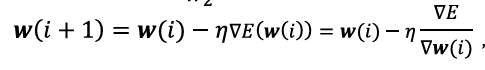
η: 학습률
∇_θL: 손실 함수에 대한 파라미터의 미분값

종류	설명
배치(Batch)	전체 데이터에 대한 평균 오차 기반 갱신
확률적(Stochastic)	샘플 하나마다 즉시 갱신
미니배치(Mini-batch)	일부 샘플 묶음 단위로 갱신 (현실적 최선)

4.3 역전파 (Backpropagation)

출력층에서부터 입력층까지 오차를 역전파하여 각 층의 가중치 갱신
체인 룰(chain rule) 기반의 연쇄 미분 구조
두 단계 구성:
1. Forward propagation: 예측값 계산
2. Backward propagation: 오차 역전파 → 가중치 업데이트

5. 🔍 핵심 정리

항목	요약
ANN의 기본 원리	뉴런 단위 계산, 가중치 조정 통해 학습
퍼셉트론 한계	비선형 문제(XOR 등) 해결 불가 → 다층 구조 필요
다층 신경망(MLP)	은닉층 통해 복잡한 비선형 관계 학습 가능
손실 함수 설계	분류/회귀 목적에 따라 다름 (MSE, CE 등)
경사하강법 + 역전파	딥러닝 학습의 핵심 알고리즘 구조

📘 강의 요약: 인공신경망(Artificial Neural Networks, ANN)

1. 🧠 ANN 개요

생물학적 뉴런을 모방한 계산 모델
입력 → 가중치 합산 → 비선형 활성화 함수 → 출력
뉴런 간 연결 가중치가 학습된 정보를 저장함

2. 🔹 퍼셉트론(Perceptron)

단층 신경망 구조
선형 결합 + 활성화 함수(step) 사용
AND, OR 문제는 해결 가능하지만 XOR 같은 비선형 문제는 불가능
→ 이를 해결하기 위해 다층 신경망(Multi-Layer Neural Network, MLP)이 필요

3. 🧱 다층 신경망(MLP)

입력층, 은닉층(hidden), 출력층으로 구성
각 층은 가중치 × 입력 + 바이어스 → 활성화 함수를 거침
대표적인 활성화 함수: Sigmoid, ReLU, Softmax 등

4. 🎯 학습 알고리즘: 손실 함수 + 경사하강법

✅ 손실 함수 (Loss Function)

유형	활성화 함수	손실 함수
회귀	항등 함수	MSE (Mean Squared Error)
이진 분류	시그모이드	크로스 엔트로피(Cross-Entropy)
다중 분류	소프트맥스	크로스 엔트로피(Cross-Entropy)

5. ⛏️ 경사하강법 (Gradient Descent)

손실 함수의 기울기(gradient)를 따라 가중치를 갱신
확률적 경사하강법(SGD)은 개별 샘플마다 업데이트 수행
배치 GD는 전체 데이터 기반, 미니배치 GD는 일부 묶음 단위로 수행

6. 🔁 순전파 & 역전파 (Forward & Backward Propagation)

순전파: 입력 → 뉴런 통과 → 출력 → 손실 계산
역전파: 오차를 출력층 → 은닉층 순으로 전달하며 가중치 갱신
역전파는 연쇄 법칙(chain rule) 기반의 델타(δ) 전파 구조

📌 Cross-Entropy와 KL Divergence 관계 정리

❓ 왜 크로스 엔트로피가 KL Divergence를 최소화하는가?

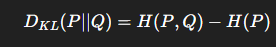
1. KL Divergence 정의

두 확률분포 P(x) (실제 분포)와 Q(x) (예측 분포) 사이의 차이를 측정하는 지표:

→ 여기서 첫 항 ∑xP(x)log⁡P(x)는 P에만 의존하므로 모델 학습과 무관

2. 크로스 엔트로피 정의

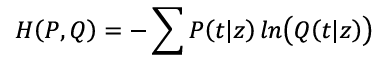
→ 이는 위 KL Divergence의 두 번째 항의 부호만 바꾼 형태

✅ 핵심 정리

H(P): 고정된 값 (타겟 데이터 분포에만 의존)
따라서, KL Divergence를 최소화하는 것은 곧 Cross-Entropy를 최소화하는 것과 동일함

💡 실전 적용: 이진 분류 (Binary Classification)

타겟 y ∈ {0,1}, 모델 예측 확률 y^ ∈ [0,1]
크로스 엔트로피 손실 함수:

이는 실제 타겟 분포 P, 예측 분포 Q 간의 KL Divergence 최소화로 해석 가능

✅ 요약

항목	정리
크로스 엔트로피 목적	예측 확률 분포가 실제 분포와 최대한 유사하도록 학습
KL Divergence와의 관계	Cross-Entropy 최소화 ↔ KL Divergence 최소화
모델 학습 의미	확률적 예측을 통해 정답 분포와의 거리(정보 차이)를 최소화

📘 인공신경망(ANN) 강의 요약

1. 🧬 생물학적 뉴런에서 영감을 받은 인공 뉴런

인공신경망(ANN)은 생물학적 뉴런 구조를 모방하여 설계됨.
입력 수용체(수상돌기) → 가중치 합산(핵) → 출력 전달(축삭, 시냅스) 구조를 기반으로 함.
입력 특징을 받아들인 후, 가중치 기반 합산 → 활성화 함수에 따라 출력 결정

2. 🔹 퍼셉트론(Perceptron): 선형 분류기의 기본 형태

단일 계층 구조, AND/OR 등 선형 분리 가능한 문제 해결 가능
한계: XOR 문제 등 비선형 문제는 해결 불가능
→ 은닉층(hidden layer)을 포함하는 다층 신경망(Multilayer Neural Network) 필요

3. ⚙️ 퍼셉트론의 학습 알고리즘

오차 수정 학습(error-correction learning) 방식
두 가지 오차 상황: 잘못된 클래스 예측
- 예: 실제 -1인데 +1로 예측한 경우 → 가중치 감소
- 예: 실제 +1인데 -1로 예측한 경우 → 가중치 증가
가중치 갱신 공식:

w(t+1)= w(t) + η ⋅ y ⋅ x

η : 학습율
y : 실제 정답
x : 입력값

반복적으로 오차가 줄어들며 수렴하는 구조

4. 📊 손실 함수 (Loss Function)

모델 예측값과 실제값 간의 차이를 수치화
회귀: 평균 제곱 오차(MSE)
분류: 크로스 엔트로피(Cross-Entropy) 사용

5. 🔍 크로스 엔트로피와 KL Divergence 관계

정보이론 기반 이론적 근거
두 분포 P (정답)와 Q (모델 출력) 사이의 KL Divergence는 다음과 같음:

여기서 H(P, Q)는 크로스 엔트로피
H(P) : 고정된 값이므로, 모델 최적화는 결국 크로스 엔트로피 최소화와 동일
즉, 크로스 엔트로피를 최소화함으로써 KL Divergence도 최소화하게 됨

6. ⛏️ 경사하강법 (Gradient Descent)

목적: 손실 함수의 기울기를 따라 가중치를 최적화
기본 공식:

종류:
- 배치 GD: 전체 데이터 기준, 안정적이지만 느리고 메모리 사용 큼
- 확률적 GD (SGD): 샘플 단위, 속도 빠르고 지역 최소 탈출 가능
- 미니배치 GD: 배치와 SGD의 절충안

7. 🔁 순전파 & 역전파 (Forward & Backpropagation)

📌 순전파 (Forward Propagation)

입력 → 가중합 → 활성화 함수 → 출력 생성
출력과 정답 간 오차 계산 → 손실 함수 반환

📌 역전파 (Backpropagation)

손실 함수에 대한 편미분을 통해 기울기 계산
연쇄법칙(chain rule)을 통해 각 층의 가중치 업데이트
심층 신경망 학습을 가능하게 하는 핵심 알고리즘

8. 🧱 다층 퍼셉트론과 비선형 문제 해결

XOR과 같은 비선형 분류 문제는 은닉층이 있는 MLP 구조로 해결
각 은닉층은 비선형 활성화 함수를 통해 고차원 표현을 학습
신경망이 복잡한 결정 경계를 학습할 수 있도록 함

📌 요약 표

항목	설명
신경망 구조	생물학적 뉴런 기반의 입력-가중합-활성화-출력 구조
퍼셉트론	선형 분류만 가능, XOR 문제 등 한계 존재
손실 함수	회귀: MSE / 분류: Cross-Entropy
KL Divergence	Cross-Entropy 최소화 ↔ KL Divergence 최소화
경사하강법	손실 기울기를 따라 가중치 갱신
SGD	메모리 효율 높고 지역 최적 탈출 가능
역전파	연쇄법칙 기반 기울기 전달, 층별 가중치 업데이트
다층 구조	은닉층을 통해 비선형 문제 해결 가능

00:00:01 In this lecture, we will learn artificial neural networks. Let's start with a general introduction to artificial neural networks. And what is the artificial neural network? The ANNS are computing systems inspired by biological neural networks that constitute animal brains. So the ANS are massively parallel distributed processors made up of simple processing units participants. In the ANS knowledge is acquired by the networks through a learning process. Specifically interneuron connection weights are used to store the acquired

00:00:58 knowledge. So the most ANNS are nonlinear input output mapping process. So as I mentioned before the ANS are inspired by the biological neuron. So let's see the biological neuron. So this is an image for the biological neuron. So you can see that it consist of multiple dendrites, nucleus, axon and then synapse. Now let's see how the neuron pass the information to the next neuron. First the dendrid takes information from the different previous neurons. Then the necross merge the information and then process the new

00:02:01 information. Then the axon will pass the processed information to synapse. Finally, the synapse pass the information to the next neurons Android. So this is the biological neuron. Then let's make an artificial neuron networks by mimicking the biological neuron. We first need some nodes to take input information like dendrates or biological neuron. Then the inputs of the different nodes will be merged according to their weight. The next node decided that the merge information should be passed or

00:02:58 not. Finally according to the decision the artificial neuron generate output. Recall the merged function of the input data like nucleus as propagation function and we call the decision function as activation function. Because according to the function the merged information will be active or not. The perceptron and the most of neural networks we will use the linear weighted combination of input as the propagation function. And please remember that we will use the host components of input as the

00:04:00 bias. And in perceptron we will use this kind of step function for the activation function. So if the merged information is larger than ARPA the information will be active by the activation function like this. However the margin information is less than the R power the information will be deactive like this. So we can simply express the perceptron with two function of x propagation function and the activation function. So we can simply express the perceptron with two function of x propagation function and the activation

00:04:57 function. From now let's simplify the perceptron. First we can simply express like this by merging the propagation and the activation functions. So only if the weighted sum of the input is larger than alpha the information will be active. And for the better visualization we can omit the propagation and the activation function like this. So finally we have some nodes for input and arrays and the output. Please don't forget that there are still a propagation and activation functions. So now let's see how we can use the

00:06:00 perceptron for classification problems. So let's see an example. Let's suppose that there are two input features X1 and X2 in the example and we set the weights. So bias and the input features like this. We also set the activation function like this. So the activation function has zero value for the alpha. That means if the propagated information is larger than zero, the information will be active and otherwise the information will not active. Finally, we will use the weighted sum of inputs for the

00:07:03 propagation. Then let's see what will be happened in the 2D feature space. So we can draw this kind of linear function when the weighted sum of input is zero. Then the area under the function will be larger than zero and upper parts of the function will be less than zero. Then according to our activation function only the area under the linear function will be active like this. So in this example you can see that the perceptron models the decision boundary or classification. So with the perceptron

00:08:07 you can solve end and war problems. In the end problem, you need to classify this lead dot from the other white dot. And in case of the or problem, you need classify these three red dots from this white dot. So I think you can simply and manually model your perceptron to find this kind of decision boundary for end and or problem. However, let's see the XR problem. In the XR problem, you need to classify these two lead dots from these two white dots. So this is a nonlinear problems. So in this case you need to

00:09:13 find this kind of nonlinear decision boundary. However our perceptron is linear model. So the perceptron can't find this kind of nonlinear function. So that's the limitation of perceptron. Actually the most of the real world problems are nonlinear. So we cannot solve the problem based on the perceptron. Because of the limitation we need to use multilayer neural networks. So now let's see how we can train our neural networks. Please remind the perceptron model we learned earlier. The perceptron is a basic neural network

00:10:13 model mimicking the human brain neurons. So we learn that it consists of input propagation activation functions and output. From now let's generalize the perceptron training algorithm or the binary classification. So let's mathematically design the problem. So to model the perceptron we first have some training data and please note that this I represent the expression of model update. Our goal is to find the weights of perceptron related to the input vector vector. And for the binary classification we

00:11:14 will use this activation function. So according to the activation function if the weighted sum of input is larger than zero the model will output one and otherwise the model will output the minus one. So let's see how we can find the proper weights for this binary classification problem. There is only two training loops. The first one is we will start a randomly chosen weights and the next one is we will update the weights to reduce the model error. Then what is the error in our problem? In the binary classification

00:12:18 problem there are two errors. Let's see the first case. Our model estimate that the label of X is one. However, in this case, the real label is minus one. So there is error. On the other hand, in the next case, our model estimated that the label of X is minus one when the actual label is one. So there are two cases how the error occurs in the problem. So in the first case if you use this update l we can reduce the error. So this time is learning late which has a value between zero and one. So according to the rule you you

00:13:32 will update the weight with the previous weight minus the learning rate multiply by the input. So now let's suppose that you update the weight according to the this update loop. Then your perceptron will estimate the output label based on weighted sum of updated weight and the input. Now let's put this term to the updated weight then you can get this equation. And then if you distribute this x to here and here then you can get this equation. Now let's see this term. You know that this is our previous

00:14:41 estimation like this. And you will see that this term is always negative because this is always positive because this is x² and this term is also always has a value between zero and one. So according to this update rule our estimated value will be always reduced according to this term. Now let's go back to here. In here we want to reduce this value because the true label is negative. And this update rule always reduce this value. So according to this update rule, our model will reduce the error during every

00:15:50 iterations. Now let's see the next case. In the next case, we can use this update loop. Same as the previous one, we can change this term to this term. And you can find that this term is always positive unlike the previous one. So according to the update rule, our model always increase the estimation value to find the positive label. So actually we can simplify the two different case with this equation. So according to the equation if there is no difference between the real label and our estimated

00:16:56 label then this term will be zero. So there is no updates on the weights. However, if there are difference like previous cases, the weights will be updated according to their direction. So this is update loom for perceptral because we update weight to reduce the model error. We can call it as error collection learning load. However, the perceptron training algorithm has limitations. We know that the perceptron training algorithm can coverage if the training data is linearly separable like and or or problems.

00:18:01 However, it can fail to coverage if the examples are not linearly separable like Sor problems. To solve the problem, we need more complex networks and alternative training algorithms. So the concept of multi-layer neural networks is proposed. You can see that there is perceptron like this and by combining the perceptron and then stacking the layer we can generate the multi-layer neural networks. Please remind that the perceptron mimics our brain's neuron. So the multi-layer neuron networks will mimic our brain that

00:19:03 consist of multiple neurons. So in the multi-layer neuron network there is input layer and output layer like proceed. And we call the middle layers as hidden layers. So let's train the multi-layer neuron networks. To train the networks, we need two things. First, we need to measure the errors of the networks. We will call them as loss functions. You can also call them as cost functions or error functions. Next we need training lose. So in this training we use gradient descent approaches for the

00:20:09 training. Let's first talk about the loss functions. Loss functions are used to determine the errors between the output of our networks and the given target values. So it will measure how well your networks model your data set. So we can call them as cost functions or error functions as I mentioned before. as they are the measure of errors. So if your predictions are totally off, your loss function will output a higher number. On the other hand, if they are pretty good, it will output a lower number.

00:21:05 So in optimization problems our goal is minimizing the loss. Now let's check the loss function in the regression problems. If you are not familiar with the concept of the regression, please first see the next video entitled as classification and regression. Before that please remind that every outputs of the perceptron will have the activation functions. So the errors of the neuron networks are related to the activation functions of the last output layer. In the regression problem, we will use the identity activation function for the

00:22:04 last up layer because the goal of the regression is estimating the continuous value. In regression, we will use sum of scaled errors as loss functions. So this y represent our target value and this y hat represent estimated values of our model. So this term will represent the distance or errors between the target value and our estimated value. Finally, if we sum the distance of every sample data, we can make the loss function. You don't need to consider this term because this term is only used for easy calculation in the future step.

00:23:20 Now let's see the loss functions for binary classification problem. In the binary classification we will use this kind of logistic sigmoid activation functions. The law of this activation function is converting the input value to the probability. We will see more details of this activation function related to the loss functions in the binary classification. In the binary classification, we can use the cross entropy loss function. Please remember that we briefly checked what the cross entropy is in the second

00:24:21 lecture. In the second lecture, we talked about the information theory. In the lecture we learned that a k divergence is a measure of the difference between two distribution P and Q. then related to the binary classification. Please suppose that this P represent the probability of the target value and this Q will represent the probability of our estimated value. Then the goal of our model is minimizing the difference between the two disrion. So we want to minimize this KL divergence. Based on the information

00:25:23 theory, the KL divergence will represented by this equation. So our goal is minimizing this equation. In the equation only this term is related to our model and we don't need to care about this term. So we call the second term as cross entropy. So our goal is changed to minimize the cross entropy with respect to Q that is equivalent to minimizing the KL divergence. Then let's go back to the binary classification and think about the cross entropy with the logistic sigmoid function. So according to the expectation of some

00:26:34 functions which I mentioned in the second lecture the cross entropy will be converted by this term. And I mentioned that the law of this logistic sigmoid function is converting the input to the probability value. So please remind that this is our model. So in in this model if we apply the sigmoid function to the upper node then the sigmoid function will convert the input value C to the probability of the output that is represented by the probability distribution. So the Q is the probability that the model estimates

00:27:40 that the Z is belong to the class one and I mentioned that this P is the probability of the real target value. So finally we can represent the cross entropy with this equation. So we can expand this summation for every t value. So it can be one or zero. So we can get this data. So as this is final pification if we set one of them as y the other will be 1 minus y. So, so we can get this term for the cross entropy. This is why we get this equation for the cross entropy loss in binary classification.

00:28:58 For multiclass classification we will use softmax activation function and this cross loss. Just think that they are generalized versions of logistic sigmoid functions and cross entropy or multiclass classification. Now let's learn about the training rules for the neural network training. So the goal of the training rule is minimizing the loss by updating our model. So now let's suppose that we have this kind of loss function. And also suppose that the weight of our model in the current stage I is this

00:30:05 one. Then in the current stage I we have to decide that we need to decrease the weight or increase the weight to minimize the loss. So that means we need to determine the direction of weight update in the current stage. Please note that we don't know the shapes of the loss exactly in that case how we can know the direction of the weight update. Now let's measure the differentiations of the loss according to our current weight. Then we can get the gradient of the loss like this lead dot line at this

00:31:13 point. By measuring the gradient we know that we can reduce the growth according to this direction. and then we will update the weight with this direction. Now we can represent the concept with this equation. Now we know that distraction is the negative gradient and we know that this is learning latent how much reduce the loss. Then by the equation we will increase the current stage weight with the learning rate and the gradient. According to our problem, we can have more complicated loss function like

00:32:19 this. So in this case, according to the starting point of the weight, the result will be changed. Let's suppose that we start at here then we can minimize the loss at this point. However, if we start at this point, then we can get the minimized loss at here. So actually we have to get the minimize loss but if we start at this point we only reach to here. So we can call it as local optimal point. Also we can extend the loss with the additional weights. In that case this term becomes vectors of the

00:33:36 weights and with the partition derivate we can get the gradient of each weight. Now let's talk about stoastic gradient descent that is opposite concept of batch. In the batch approach the weights are updated once that is after all the training examples have been passed through the networks. On the other hand, in the stoastic gradient descent, the parameters are updated after computing the loss of each individual training samples respectively. So this is concept of online learning. So this is an example of batch

00:34:35 and stoastic gradient effect. In the batch approaches, we first see the all the training examples and then measure the loss. In that case, the weights are updated to the direct direction to the local optima. In the sastic gradient descent, we compute the loss of each training sample respectively. So when we see the first sample, we know that this point is the right direction. However, when the we see the next sample, we know that this point is the right point. So after every iteration, we find the

00:35:41 direction like this. The first advantage of the scopastic presented descent is that is easier to fit into memory. In case of batch, we have to upload every samples to the memory. However, in the most case, we have a lot of training samples. So in that case, we will suffer memory problems. However, in the stoastic gradient descent approaches, we only need to upload just a single samples to the memory for every iteration. Also, we only measure the loss for single train sample for every iteration. It is computationally fast.

00:36:42 The most important things is it can help getting out of local minima in the batch app. We directly update weight to here. However, let's suppose that this point is a local optima. In that case it is very hard to get out of here with the batch approaches. However, in case of the stoastic gradient descent, we will have chance to get out of this local minima by following the different direction according to the sample. However, because of that, it may take longer to achieve the convergence. Now let's see how we can

00:37:48 train deep neural network. We use two propagation in the training. So first one is forward propagation. The next is backward propagation. which we called back propagation. So now let's see them one by one. Actually you already saw the for propagation. So if we have input we perform weighted sum of the input and apply the activation function then we can get the output. This process is forward propagation. Now let's represent process with more details. First we can represent the f function which is the

00:38:55 linear combination of the weight and input as a and we can represent the activation function g like this one. So after applying the activation function to the A we can get output G. So in the forward propagation we pass the input information through the networks to the output. And if we get the output according to the input we can measure the loss function. So this is loss function and also please remember that we need to measure the gradient with particial deviation of the loss function to update our weight in the

00:40:13 training l. So this one in the previous page by using the chain rule we can separate this term to this one. We first convert the first term to the delta. Now let's see the next part. A is the linear combination of weight and Z. So if we derate A with the weight, we can only get the C. Let's see more details about the delta. Then this delta is this one. And by using the channel we can represent the data like this. Now we can see the delta of the next layer at here. So it means we can represent the delta

00:41:34 at the L layer to the summation of the next layers delta. Now let's see the next term. By using the chain rule we can represent this one with this one. So in the first term we see that we derate the a according to the c then we can get the w at here and if we calculate this term we will get this one. So finally we can express the delta term to this one and the next two layer delta and this weight respectively. This is summary of forward and backward propagation. In the fourth propagation, we'll pass

00:42:49 the information of the previous layer with propagation and activation functions. And in the back propagation, the error will be passed to the previous layer with delta function for neural network training. Now let's see a brief overview for training the neuronal networks. In word propagation the input information is passed through the neuron networks and the neuron networks finally estimate outputs by comparing the estimated output and the true label with loss function. We measure the error of the

00:43:39 neuron networks and the error will be passed to the previous layer step by step with delta function in back propagation and during the back propagation weight of each layer will be updated to reduce the error. So if you have any question please contact me by this email. Thank you.

Summary

This lecture provides a comprehensive introduction to artificial neural networks (ANNs), starting from their biological inspiration and basic unit—the neuron—to more complex structures and training methodologies. ANNs are computing models inspired by the neurons in animal brains, built as massively parallel processors composed of simple interconnected units. The lecture explains how biological neurons receive, process, and transmit information, and then maps these biological processes to artificial neurons, highlighting core elements such as dendrites, axons, propagation (weighted sums), and activation functions.

A fundamental ANN model—the perceptron—is introduced as a simple linear classifier capable of solving linearly separable problems like AND and OR, but limited in handling nonlinear problems such as XOR. This limitation motivates the extension to multi-layer neural networks, which incorporate hidden layers to capture nonlinearity.

The lecture details the perceptron training algorithm for binary classification, focusing on weight updates guided by minimizing the classification error through an iterative learning process. It discusses error cases, how weights are adjusted via a learning rate, and the importance of convergence conditions.

Further, it explains the importance of loss functions to quantify the difference between model outputs and targets, with examples from regression (sum of squared errors) and classification (cross entropy with logistic sigmoid or softmax activation). The cross entropy loss is tied back to information theory concepts such as Kullback-Leibler divergence, illustrating its theoretical foundations.

Key training methods, specifically gradient descent and variants like stochastic gradient descent (SGD), are explained, emphasizing the use of gradients to determine the direction of weight updates aiming to minimize loss. The lecture differentiates between batch and stochastic updates, highlighting SGD’s advantage in managing memory, computational efficiency, and escaping local minima while noting its slower convergence.

Finally, training of deep neural networks through forward and backward (backpropagation) propagation is detailed. Forward propagation computes outputs from inputs through layers via weighted sums and activation functions, while backpropagation propagates error gradients backward to update weights using the chain rule, enabling the network to learn effectively over multiple layers.

Overall, this lecture lays a foundational understanding of neural network structure, learning principles, loss functions, optimization techniques, and training procedures necessary for more advanced deep learning research and applications.

Highlights
🧠 Artificial Neural Networks (ANNs) are inspired by biological neurons, mimicking their structure and function.
⚙️ The perceptron is a simple neural model effective for linear classification problems like AND/OR but limited for nonlinear tasks like XOR.
📉 Training involves updating weights iteratively to minimize classification error using error correction learning with a learning rate.
🧮 Loss functions, including sum of squared errors for regression and cross entropy for classification, quantify model performance.
🔄 Gradient descent and stochastic gradient descent optimize model weights; SGD is more memory-efficient and helps escape local minima.
↔️ Forward propagation computes outputs while backpropagation updates weights by propagating error gradients backward.
🏗️ Multilayer neural networks with hidden layers address perceptron limitations, enabling learning of complex, nonlinear decision boundaries.
Key Insights

🧬 Biological Inspiration Lays the Groundwork for ANN Design: Understanding the biological neuron’s dendrites, axon, and synapse helps conceptualize data flow and signal processing in artificial neurons, fostering more intuitive neural network architectures.

🔍 Perceptron Highlights Importance and Limits of Linear Models: Though powerful for linearly separable data, perceptrons cannot solve nonlinear problems (e.g., XOR), underscoring the need for more complex networks or nonlinear activation strategies in real-world applications.

🔄 Weight Update Rules Minimize Model Error Through Iterative Learning: The perceptron’s weight update algorithm uses calculated errors to adjust weights systematically, ensuring that the model progressively makes fewer mistakes on training data, an essential principle in supervised learning.

📊 Loss Functions as Objective Metrics Drive Training: Proper selection and understanding of loss functions (e.g., cross entropy for classification) are crucial because they directly impact optimization effectiveness, guiding model predictions closer to true label distributions.

📉 Gradient Descent and Its Variants Are Core Optimization Tools: Gradient-based methods exploit the differentiable nature of neural networks to efficiently move weights towards minimizing loss, making these algorithms fundamental in deep learning practice.

⚖️ Stochastic Gradient Descent Offers Practical Advantages Despite Noise: Although updating weights sample-by-sample introduces variance and longer convergence, its reduced memory footprint and ability to escape poor local minima solidify SGD as a predominant training method.

🔁 Backpropagation Unlocks Deep Learning by Enabling Weight Updates Across Layers: Applying the chain rule to propagate error gradients enables the training of multilayer networks efficiently, allowing deep architectures to learn hierarchical feature representations vital for complex tasks.

This structured overview provides a solid foundation for understanding artificial neural networks, their challenges, and training mechanisms pivotal to the broader field of machine learning and artificial intelligence.

5강 - 딥러닝에서 정규화

📌 개요: 정규화(Regularization)의 필요성

딥러닝 모델은 매우 복잡하고 수많은 파라미터를 포함하므로 과적합(Overfitting) 문제가 자주 발생합니다. 과적합은 학습 데이터에는 잘 맞지만 테스트 데이터에는 성능이 떨어지는 현상입니다. 이를 해결하기 위한 다양한 정규화 기법이 소개됩니다.

1. Underfitting vs Overfitting

Underfitting: 모델이 너무 단순하여 학습 데이터조차 제대로 설명하지 못함.
Overfitting: 모델이 너무 복잡하여 학습 데이터에만 최적화되고, 새로운 데이터에 일반화되지 못함.
목표: 일반화 성능이 높은 "Just Right" 모델을 찾는 것.

2. 신경망 학습을 위한 정규화 접근법

정규화 기법	주요 역할
Early Stopping	검증 성능이 더 이상 개선되지 않으면 학습 중단
Momentum	진동을 줄이며 빠른 수렴 유도
Adaptive Learning Rate	각 파라미터에 맞는 학습률 자동 조정
Norm Regularization	모델 복잡도 제한 (L1, L2)
Dropout	무작위 뉴런 제거를 통한 앙상블 효과 유도
Batch Normalization	층별 입력 분포 정규화로 학습 안정화

3. Early Stopping

개념: 검증 데이터 손실이 증가하면 학습을 조기에 멈춤.
목적: 과적합 방지, 불필요한 추가 학습 방지.

4. Momentum 기법

SGD는 지그재그식 진동 발생 가능 → 관성(moving average) 개념 도입.
Momentum 방식:

Nesterov Accelerated Gradient (NAG): 한 단계 앞을 미리 고려한 업데이트.

5. Adaptive Learning Rate

각 파라미터마다 개별 학습률을 조정하여 최적화를 향상시킴.

Adagrad: 자주 업데이트되는 파라미터에 대해 학습률 감소.
RMSProp: Adagrad의 과도한 감소 문제를 해결 (지수이동평균 도입).
AdaDelta: 학습률 자체를 없애고 변화량 기반으로 조정.
Adam: Momentum + RMSProp 결합, 가장 널리 사용됨.

6. Norm 기반 정규화 (Weight Regularization)

손실 함수에 L1, L2 정규화 항을 추가하여 모델 복잡도 제어.

L1 정규화 (LASSO): 가중치의 절댓값 합 → 희소성 유도 (feature selection 효과)

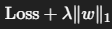
L2 정규화 (Ridge, weight decay): 가중치 크기 제한 → 매끄러운 일반화

7. Dropout (JMLR 2014)

학습 중 무작위로 일부 뉴런을 비활성화 (0으로 masking)
다양한 신경망을 앙상블 학습하는 효과
테스트 시에는 전체 뉴런을 사용하되, dropout 확률에 맞게 scaling

8. Batch Normalization

각 레이어의 입력을 미니배치 기준으로 정규화

효과:
- 내부 공변량 변화 감소
- 학습 안정성 및 속도 향상
- Dropout 없이도 과적합 완화 가능

9. Vanishing Gradient 문제

Sigmoid, Tanh 사용 시 깊은 신경망의 초기 층에서 gradient가 사라짐
해결책:
- ReLU, ELU 등의 활성화 함수 사용
- BatchNorm, Residual 구조, He 초기화 등 보완 기법 활용

🧠 종합 요약

분류	기법	역할 및 핵심 개념
최적화 보조	Momentum, Adam	빠른 수렴, 지그재그 방지, 학습률 자동 조정
과적합 방지	Early Stopping, Dropout	학습 중단 시점 판단, 뉴런 무작위 제거로 앙상블 유도
일반화 성능 향상	L1, L2 Regularization	가중치 제한, 희소성 유도, feature 선택
안정적 학습 지원	Batch Normalization	분포 정규화, 학습 가속화 및 Vanishing Gradient 완화
깊은 네트워크 안정화 및 확장	ReLU, ELU 등	활성화 함수 선택으로 gradient 소실 완화, 비선형성 확보

✅ 결론

정규화는 단순한 성능 향상 기술이 아니라, 딥러닝 모델이 실제 환경에서 일반화된 성능을 보장하도록 만드는 필수 구성 요소입니다.

📌 정규화 강의 대본 기반 심화 요약

1. 과적합/과소적합 상태를 손실 그래프로 진단하는 방법

Underfitting:
- 훈련 손실과 검증 손실이 모두 높음 → 모델이 학습 자체를 잘 하지 못함.
Overfitting:
- 훈련 손실은 낮지만 검증 손실이 증가 → 모델이 학습 데이터에 과하게 적합됨.
진단 방법: 학습 도중 손실 그래프 추세를 통해 어느 시점에서 과적합이 시작되는지 감지 가능.

✅ 학습 중 손실의 변화 패턴을 통해 조기 종료(Early Stopping) 시점을 파악할 수 있는 실질적 기준을 제시함.

2. 모멘텀 기반 최적화 시 직관적 업데이트 경로 설명

Momentum SGD의 효과:
- 손실 함수가 길고 좁은 골짜기 모양일 경우, 일반 SGD는 지그재그로 느리게 수렴함.
- 이전 단계의 속도(gradient 방향 누적)를 활용하면 빠르게 최적점에 접근 가능.
- 속도 벡터는 이전 gradient의 방향성과 현재 gradient의 크기를 적절히 조합함.

✅ 실제 loss surface의 형태를 고려할 때 Momentum이 가지는 실질적 장점을 직관적으로 이해시킴.

3. Adaptive Learning Rate 계열 기법의 수학적 직관

알고리즘	핵심 아이디어
Adagrad	자주 업데이트되는 파라미터의 학습률 감소 → 역학습률 효과
RMSProp	Adagrad의 누적 제곱 누적 문제를 지수이동평균으로 보완
AdaDelta	학습률 자체를 없애고, weight 변화량의 제곱 평균으로 scaling 수행
Adam	Momentum + RMSProp → 가장 일반적인 Adaptive Optimizer

✅ 학습률이 각 파라미터별로 어떻게 동적으로 조절되는지, 수식 내에서 어떤 항이 영향을 주는지 설명함.

4. Norm 기반 정규화 (L1 vs. L2) 미분 및 업데이트 동작 상세 비교

L1 (LASSO)

업데이트 시, 파라미터의 부호만 고려해 일정량 감소/증가함 → 희소성(sparsity) 유도
도함수: 파라미터 값이 양수면 -λ, 음수면 +λ

L2 (Ridge)

파라미터 크기에 비례하여 감소/증가함 → 크기 자체 제어, 부드러운 감소
도함수: λ * w 형태로 weight 자체의 크기에 따라 업데이트됨

✅ L1은 0에 가깝게 수렴 → feature selection 효과, L2는 큰 weight 억제 → 안정화. 두 방식의 미분 구조 차이를 수식적으로 비교함.

5. Dropout의 학습 시 동작 방식 구체화

매 iteration마다 일부 뉴런을 확률적으로 제거하여 부분 네트워크만 학습.
실제 구현:
- 학습 중: 뉴런을 확률적으로 비활성화
- 추론 시: 전체 뉴런 활성화 + weight scaling

✅ Dropout이 앙상블처럼 작동하며 regularization 효과를 주는 원리를 구체적 그림으로 설명함.

6. Batch Normalization의 실제 계산 방식 요약

미니배치 단위로 평균과 표준편차 계산:

장점:
- 내부 공변량 이동(Internal Covariate Shift) 완화
- 학습 안정성 및 속도 향상
- ReLU와 함께 사용 시 성능 개선 극대화

✅ 계산 수식과 실행 위치(각 레이어의 입력)에 대해 명확히 언급하며 실전 적용을 위한 기반 제공.

7. Vanishing Gradient 문제와 활성화 함수 선택

Sigmoid:
- 도함수가 최대 0.25이며, 입력이 크거나 작을수록 gradient가 0에 수렴
- → 역전파 중 gradient가 사라지는 문제 발생
해결책:
- ReLU, Leaky ReLU, ELU 등 미분값이 0에 수렴하지 않는 함수 사용

✅ gradient 소실 문제를 수식 기반으로 설명하고, ReLU 계열 함수가 이를 완화하는 방식 명확히 기술.

📌 종합 요약

주제	핵심 내용 요약
손실 그래프 활용한 과적합 판단	검증 손실 증가 시점에서 Early Stopping 가능
Momentum SGD	진동 억제 및 수렴 가속
Adaptive Optimizers	Adagrad, RMSProp, Adam 등 파라미터별 동적 학습률 조정
L1 vs. L2 정규화	희소성 vs. 부드러운 억제, 도함수 구조에 따라 업데이트 방식 달라짐
Dropout	무작위 뉴런 비활성화로 과적합 방지 및 앙상블 효과 유도
BatchNorm	레이어 입력 정규화로 학습 안정성 향상
Vanishing Gradient	Sigmoid → gradient 소실, ReLU 계열로 완화

📘 딥러닝 정규화와 안정적 학습 기법 요약

🎯 목표

딥러닝 모델 학습에서 흔히 발생하는 과소적합(underfitting)과 과적합(overfitting) 문제를 완화하고, 일반화 성능이 우수한 모델을 구현하기 위한 다양한 정규화 및 최적화 전략을 소개한다.

🧩 핵심 정규화 및 학습 기법

1. Early Stopping

개념: 검증 손실이 상승하는 시점에서 학습을 조기에 중단
효과: 과적합 방지에 간단하면서도 강력한 방법

2. 모멘텀 최적화 (Momentum)

핵심 원리: 이전 step의 gradient를 누적 반영하여 갱신 방향을 부드럽게 유지
장점: 경사가 좁고 긴 영역에서 지그재그 움직임 감소 → 빠른 수렴, 진동 억제

3. Adaptive Learning Rate (적응적 학습률)

기법	핵심 특징
AdaGrad	자주 업데이트된 파라미터의 학습률 감소 (보수적)
RMSProp	AdaGrad 개선형, 오래된 gradient 영향 감소
Adadelta	학습률 없이 상대 변화량만으로 갱신 수행
Adam	Momentum + RMSProp 결합 → 일반적 기본 설정

공통 효과: 파라미터마다 학습률을 자동 조정 → 수렴 안정성 및 속도 향상

4. Norm 기반 정규화 (L1 vs L2)

✅ L1 정규화 (Lasso)

효과: 일부 weight를 0으로 만들어 희소성(sparsity) 유도
의의: 중요하지 않은 feature 제거 → 모델 해석성 및 효율성 증가

✅ L2 정규화 (Ridge)

효과: 큰 weight의 크기를 점진적으로 축소 → 부드러운 억제(weight decay)
의의: 과적합 완화 및 훈련 안정성 제공

5. Dropout

개념: 학습 중 임의의 뉴런을 비활성화하여 부분 모델들(앙상블)을 학습
효과:
- 특정 뉴런에 과도하게 의존하는 현상 방지
- 일반화 성능 향상
- 노이즈 또는 결측치에 대한 강인성 증가

6. Batch Normalization

개념: 미니배치 단위로 입력 분포를 정규화
효과:
- 내부 공변량 이동(Internal Covariate Shift) 완화
- 높은 학습률 허용 → 빠른 수렴
- 폭주/소실되는 gradient 문제 감소

7. Vanishing Gradient 대응

문제: sigmoid 함수는 gradient가 작아져 깊은 네트워크에서 학습이 불가능
대응: ReLU 및 변형 함수 사용
- ReLU: 0 이상 구간에서 gradient 유지
- 효과: 깊은 네트워크에서도 효과적인 역전파 가능

✨ 핵심 통찰

구분	통찰 요약
📈 Momentum	최적화 경로를 부드럽게 하여 수렴 가속 및 불안정한 진동 억제
🧮 Adaptive LR	파라미터별 이력 기반 학습률 조정으로 효율적 수렴
⚖️ L1/L2 정규화	복잡도 제어 및 일반화 향상- L1: 희소성- L2: 크기 억제
🎲 Dropout	무작위 뉴런 제거를 통한 앙상블 효과 및 과적합 방지
🧾 BatchNorm	학습 안정화 및 수렴 속도 향상
🔥 ReLU 도입	Vanishing Gradient 문제 근본적 해소 → 딥러닝 발전의 핵심 기여

✅ 결론

단순한 기법 소개를 넘어, 각 정규화 전략이 왜 필요한지, 어떤 상황에서 효과적인지, 그리고 학습 안정성과 일반화 성능 향상에 어떻게 기여하는지를 이론과 직관 모두에서 명확히 전달한다. 이러한 이해는 실제로 딥러닝 모델을 구현하고 튜닝하는 과정에서 핵심적인 의사결정에 기반이 된다.

00:00:01 in the previous lecture we learn that how we can PR our deep neural network so in this lecture we will learn that how we can well train the de neural network so I will introduce some techniques for regularization of our deep neural netor in the previous lecture we talked about Under feting and Over feting problems in the regression and classification problem during our neural network training steps we can indirectly check under feing and overfitting with decreased pattern of the loss so in case of the under feting our

00:00:59 training LS is still too high compared to the validation then means our model still not fit well to our training data like this case on the other hand in the case of overrating we can see that the training loss is too low compared to validation loss that means our model is overfit to the training data like this case so our goal is find a good model like this one so in this lecture we long how we can find this kind of Wellfit model there are lot of different method to well train your NE netor so see them one by

00:02:21 one if you use any deing tool Parts like tens of FL or py to you have to set some parameter value related to this approaches so if you learn this approaches then you can easily use that two paths and also well train your neural networks so one of the easiest way is only stopping in the most of the case you will meet the overfitting problems during the neural network training because we don't have enough data compared to your largest size model so easiest way to solve the overfitting problem is stop the training

00:03:24 in the early stages in the early stage both the training and validation loss will decrease like this but in some point the valuation loss will be increased when the training loss is decreased in that point we can say that the model is over fting so you can just start the training at the point to preserve the over fitting problem that is only stopping the other way is use momentum I hope that you can remind the stochastic gradient descent in the approach we can update our weights based on the amount of the

00:04:27 gradient so please remind this previous lecture page so so I bring this equation if we use momentum we can replace this gradient t to the velocity so the velocity T will be represented by the portion of the previous velocity and the gradient term let's see the graph the first term represent the momentum step that means the previous gradient Direction and amount and the second term represent current step of the gradient so same as this to so the velocity ter means we can decide the update Direction and the amount

00:05:38 based on the previous gradient and the current gradient so if you sequentially follow this velocit form like this then you can finally get this home now let's talk about the advantage of the momentum so let's suppose that you have this kind of long long narrow loss function so if you just use stochastic gr to desent without the momentum your loss will be decreased like this pattern that means it will oscillate according to the really and very slowly update to find the minimum loss so if you use the previous gradient

00:06:42 Direction with momentum your model will found the minimum loss very fast like this we can also well train our neural networks based on the Adaptive learning late so please remind that this is learning late in gr descent so in this case we adaptively decide the loaning late so there are some different way to assign the Adaptive learning rate so the first one is a grade so the a grade Decay The Learning L for each parameter in portion to their update history that means more updates than more Decay so in the a rate we will replace

00:07:58 this learning late like this so now let's see the G function the g means the sum of the previous G and the scale of the gradient so this one is if each parameter has larger previous gradient then the G of the parameter will be rure right and in this ter if you have larger G value the overall ter value will be smaller so a parameter has larger gradient that means more update the running rate of the parameter will be decreased like this so another way is RMS proofs so root mean Square propagation there is the same as the a

00:09:17 grade but it will use the Lambda ter and one minus Lambda to consider the ratio of G previous G and size of the gradient another way is Ada Delta Delta so a Delta we can replace the larning late parameter to the D function so let's see the equation so G function is same as the previous one but in this case we will replace the larning L ter to this one so when we see the D function it consist of the previous D function and the size of the weight different please note that this time represent the size of the gradient and

00:10:27 this represent the size size of the weight difference so when you see the distance if the weights are largely changed then we will have the r loing late the other way is at so you can just simply think that it is the THM of the momentum ands Pro so you can update your weight based on the velocity ter for momentum and the g function for RS proof let's talk about non based regularization approaches please remind that what the norm is we learned about Norm in the basic mathematics in the lecture we learned

00:11:36 that Norms are functions that measure how large a vector is so we can represent the norm with this equation so according to the P value we can call it as Aon or l so the term of eron is this one and term of a is one please note that we use the absolute value for eron and root square value for L2 nor please also remind that we learned about L function in the previous lecture so we will use this kind of loss function for our problems so in case of liation we will use mean Square anal loss function and

00:12:46 classification we will use the cross entropy loss now let's apply the Norms to our loss function so this L represent our final loss function and this e represent our arror function like in scale Arrow or cross entropy and this R represent the known ter so the E is data dependent aror ter and the r is penalty or regularization term and L is the final L function now let's first apply the ER known to this regularization ter we can call it as last one then the AL ter will represent by the arror n and as I mentioned

00:13:57 before we will use the sum of absolute value for iron nor now let's update one of the weight parameter with the final loss function L then let's measure the gradient time then we derivate this Lo function according to the weight parameter then we will get this two ter right and the first ter is our gradient of loss function without the regularization ter let's calculate a second ter so if you measure the second term we only get the Lambda or negative Lambda according to the weight value so let's think about the meaning

00:15:16 of this T so let's think that the current weight is larger than zero then we will add the negative Lambda with this sign right so we will decrease the current weight is larger than zero on the other hand if we have the negative value for the WD we will add the Lambda with this sign so in that case we will increase the current weight value so with the Aron P we will make the current weight is close to Zero by adding the Lambda or negative Lambda according to the sign of the current weights so the Aron

00:16:32 T will increase the sparity of our weight now let's talk about alome so in case of alome we will apply the Alon to the regularization term like and as I mentioned before we will use some of scale value like this now let's update our weight with the gradient of the final loss then like previous one we will get this one and this one for L2 and we can measure the this like this one now we can apply this ter to here and think about that so like if we have the positive W1 then we will reduce the value with

00:17:48 this s sign on the other hand if we have the negative value for the weight then we will increase the the weight because this one will be negative and with the negative sign the the final will be the positive so in case of the negative value we will increase the value the main difference compared to the error Nome we will increase or decrease the the W by reflecting the size of the weight so then means if we have R positive weights then we will largely decrease the weight so the low of the al2 is reducing

00:18:53 the magnitude of current weights so this is called a and weight Decay the last one is drw off the concept of drw off is very simple so let's see the standard neural network and this is fully connected to another however in this case there are a lot of weights to train in case of the Dropout approaches for every iteration we randomly select the node and only update the weights related to the selected no like this so by using the drawout we can reduce the parameter which should be run for every iteration

00:19:59 now let's talk about batch normalization during the neural netor training you will put the multiple training samples with mini batch size so the batch normalization means normalizing the inputs of each layer for each mini so it is known that if you use batch normalization then you can improve the speed performance and stability of network so actually the bch normalization step is very simple so let's suppose you have M training samples for each mini bch then you can measure the mean and standard deviation for the

00:20:54 samples and so you can just normalize every sample like this that is best normalization now let's talking about Vanishing gradient problem and the activation functions we usually use the sigmoid activation function for the activation function so the sigmoid activate function looks like this now let's see what will be happened in the back propagation step so in the previous lecture we learned that the Delta function will pass during the back propagation now let's see this one this three is activation function and we will

00:21:52 derivate the equation function now let's see theun function for the deviation of the sigo in the most case it has very small value close to zero right so during the back propagation we will pass this Delta function from last to front and the very small value will multiply sequentially so when you go very front then the stack value will be zero so wa in the front layer will not update because the gradient is vanish it that is the vanishing gradient problem to solve the problem many different type of activation functions

00:23:07 are proposed like l so in this case the derivate of the activation function is not too small so we can reduce the vanish gradient Vanishing problems so in this lecture we learn about different approaches to well train our de networks and so please be familiar with these TS and please remember the meaning of the T respectively please contact me by this email if you have any question thank you

Summary

This lecture focuses on effective training techniques for deep neural networks (DNNs), emphasizing regularization methods to avoid underfitting and overfitting issues encountered during model training. The lecturer revisits the concepts of underfitting—where the model performs poorly on training data—and overfitting—where the model memorizes training data but generalizes poorly on validation data. The goal is to achieve a well-fitted model, balancing bias and variance effectively.

Several key strategies for well-training DNNs are covered:

Early Stopping: Halting training when validation loss starts to increase to prevent overfitting.
Momentum in Gradient Descent: Incorporating past gradients to smooth updates and accelerate convergence, especially useful for navigating narrow minima and avoiding oscillations in loss function optimization.
Adaptive Learning Rates: Techniques such as AdaGrad, RMSProp, Adadelta, and Adam adjust learning rates dynamically per parameter to optimize training efficiency and stability.
Norm-based Regularization (L1 and L2 Norms): Adding penalty terms based on weight magnitudes to the loss function discourages large weights, improving generalization by promoting sparsity (L1) or weight decay (L2).
Dropout: Randomly disabling nodes during training to reduce dependency on specific weights and improve model robustness.
Batch Normalization: Normalizing inputs within mini-batches to stabilize and speed up training by addressing internal covariate shift.
Addressing Vanishing Gradient Problems: Explaining why sigmoid activations lead to gradient vanishing in deep networks and introducing ReLU and its variants that maintain steady gradients to enable effective backpropagation.

The lecture ties these regularization concepts with practical parameter tuning, especially in popular deep learning frameworks like TensorFlow and PyTorch, preparing students to implement them effectively.

Highlights
⚡ Early stopping is a simple yet powerful method to prevent overfitting by halting training at the right moment.
🔄 Momentum uses previous gradients to accelerate training and reduce oscillations in narrow loss valleys.
📉 Adaptive learning rate algorithms such as AdaGrad and RMSProp dynamically adjust parameter updates for better convergence.
⚖️ L1 and L2 regularization include penalty terms in the loss function to control model complexity and improve generalization.
❌ Dropout randomly removes nodes during training, reducing overfitting by preventing co-adaptation of neurons.
🧮 Batch normalization normalizes inputs per mini-batch, stabilizing and speeding up network training.
🚫 The vanishing gradient problem with sigmoid activations hampers deep learning; using ReLU overcomes this challenge.
Key Insights

🔄 Momentum optimizes gradient descent by incorporating past updates, allowing the model to maintain direction and speed: This approach prevents slow, zig-zagging progress through narrow minima, thereby accelerating convergence and improving training stability.

📊 Adaptive learning rate methods enhance training by customizing step sizes per parameter based on historical gradient information: For example, AdaGrad reduces learning rates for parameters with large gradients, preventing overshooting, whereas RMSProp improves this by limiting the accumulation of squared gradients, thus avoiding aggressive decay.

🏋️‍♂️ L1 regularization promotes sparsity by pushing some weights exactly to zero, potentially leading to more interpretable and efficient models: The penalty term adds or subtracts a fixed value from weights depending on their sign, effectively pruning less important features.

🌱 L2 regularization (weight decay) discourages large weights by shrinking all weights proportionally to their size, helping the model avoid overfitting: Unlike L1, L2 does not generate sparsity but results in smooth weight distributions that generalize better.

🌀 Dropout acts as an ensemble technique by training different random subsets of neurons each iteration, improving generalization and reducing co-adaptation risk: This stochastic approach causes the model to become more robust against noisy or missing inputs.

⚙️ Batch normalization normalizes each mini-batch’s inputs to reduce internal covariate shift, making training more stable and allowing higher learning rates: This results in faster convergence and helps prevent exploding/vanishing gradients.

💡 Replacing sigmoid activations with ReLU-type functions solves vanishing gradient problems by maintaining gradients above zero for positive inputs, enabling deeper networks to learn effectively: This shift has been critical in advancing deep learning, particularly in very deep architectures.

This comprehensive overview equips learners with crucial techniques and theoretical insights necessary for successfully training deep neural networks while avoiding common pitfalls. Mastery of these concepts enhances both model performance and training efficiency in practical machine learning workflows.

저작자표시 비영리 (새창열림)

'인공지능 > 공부' 카테고리의 다른 글

딥러닝 공부하기 3 (4)	2025.07.03
딥러닝 공부하기 2 (1)	2025.07.02
시험 공부 겸 정리하는 곳 - LVLM (0)	2025.04.21
재미있는 인공지능 속 세상 여행 3주차 - Chat GPT의 등장과 비즈니스 환경 변화 (8)	2024.09.18
재미있는 인공지능 속 세상 여행 1, 2주차 - 생성형 AI (10)	2024.09.10

현재글딥러닝 공부하기 1

NLP, AI, XAI에 관심있는 공대생의 일기장...?

Today :
Yesterday :