워드 임베딩 시각화
Introduction
Chapter 4. 단어 임베딩 만들기 강의의 워드 임베딩 시각화 실습 강의입니다.
이전 실습에서처럼 (1) 단어 임베딩의 대표적인 방법인 Word2Vec을 활용하여 워드 임베딩을 직접 구축해보고, (2) 이번 실습에서는 구축한 워드 임베딩을 2차원으로 시각화하여 임베딩의 품질을 보다 정교하게 측정해보겠습니다.
이후 실습의 용이성을 위해 한국어 글꼴을 설치합니다!
!sudo apt-get install -y fonts-nanum
!sudo fc-cache -fv
!rm ~/.cache/matplotlib -rf
1. 한국어 워드 임베딩 구축
워드 임베딩 구축 과정은 지난 실습에서 다뤘으므로, 이번 실습에서는 빠르게 구축을 진행해볼게요!
오늘 사용할 학습 데이터셋은 네이버 영화 리뷰 데이터셋입니다.
네이버 영화 리뷰 데이터셋은 총 200,000개 리뷰로 구성된 데이터로, 원래 목적은 영화 리뷰를 긍/부정으로 분류하기 위해 만들어진 데이터셋입니다.
따라서, 주어진 리뷰가 긍정인 경우 1, 부정인 경우 0을 표시한 레이블로 구성되어져 있습니다.
이번 강의에서는 이 데이터셋을 활용하여 단어 임베딩을 구축해볼게요!
레이블은 사용 안합니다!

1.1. 데이터 수집
- 학습 데이터셋 경로: https://raw.githubusercontent.com/e9t/nsmc/master/ratings_train.txt"
- 테스트 데이터셋 경로 : https://raw.githubusercontent.com/e9t/nsmc/master/ratings_test.txt
import urllib.request
import pandas as pd


urllib.request.urlretrieve("[https://raw.githubusercontent.com/e9t/nsmc/master/ratings\_train.txt"](https://raw.githubusercontent.com/e9t/nsmc/master/ratings_train.txt"), filename="ratings\_train.txt")
urllib.request.urlretrieve("[https://raw.githubusercontent.com/e9t/nsmc/master/ratings\_test.txt"](https://raw.githubusercontent.com/e9t/nsmc/master/ratings_test.txt"), filename="ratings\_test.txt")

#오늘 사용할 학습 데이터를 다운로드합니다.

#원 데이터셋의 학습 데이터셋은 150,000개, 테스트 데이터셋은 50,000개인데, 데이터가 너무 크면 학습이 오래 걸리므로, 이번 강의에서는 테스트 데이터셋을 학습 데이터셋으로 활용해볼게요!

train\_dataset = pd.read\_table('ratings\_test.txt')
print(len(train\_dataset)) # 50000

train\_dataset\[:5\]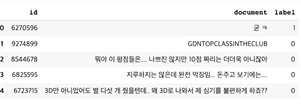
1.2. 데이터 전처리
데이터셋 다운로드가 완료되었으니, 이제 데이터를 분석하고 간단한 전처리를 진행해볼게요
1.2.1. 데이터셋 내 결측값 확인
train\_dataset.replace("", float("NaN"), inplace=True)
print(train\_dataset.isnull().values.any()) # True

train\_dataset = train\_dataset.dropna().reset\_index(drop=True)
print(f"필터링된 데이터셋 총 개수 : {len(train\_dataset)}") # 49997
1.2.2. 데이터셋 내 중복 데이터 제거
# 열을 기준으로 중복제거

train\_dataset = train\_dataset.drop\_duplicates(\['document'\]).reset\_index(drop=True)
print(f"필터링된 데이터셋 총 개수 : {len(train\_dataset)}") # 49157
1.2.3. 한글이 아닌 문자를 포함하는 데이터 제거
# 정규 표현식을 사용하여 한글이 아닌 문자 제거

train\_dataset\['document'\] = train\_dataset\['document'\].str.replace("\[^ㄱ-ㅎㅏ-ㅣ가-힣 \]","")
train\_dataset
1.2.4. 길이가 너무 짧은 데이터 제거
# 문서 내 길이가 너무 짧은 단어를 제거합니다. (단어의 길이가 2 이하)

train\_dataset\['document'\] = train\_dataset\['document'\].apply(lambda x: ' '.join(\[token for token in x.split() if len(token) > 2\]))
train\_dataset
1.2.5. 전체 길이가 10 이하이거나 단어가 5개 이하인 데이터 제거
# 전체 길이가 10 이하이거나 전체 단어 개수가 5개 이하인 데이터를 필터링합니다.

train\_dataset = train\_dataset\[train\_dataset.document.apply(lambda x: len(str(x)) > 10 and len(str(x).split()) > 5)\].reset\_index(drop=True)
train\_dataset # 이번에는 긴 애들이 남는다.
1.2.6. 한국어 불용어 제거
!pip install konlpy

from konlpy.tag import Okt

# 불용어 정의

stopwords = \['의','가','이','은','들','는','좀','잘','걍','과','도','를','으로','자','에','와','한','하다'\]

train\_dataset = list(train\_dataset\['document'\])

# 형태소 분석기 OKT를 사용한 토큰화 작업

okt = Okt()

tokenized\_data = \[\]

for sentence in train\_dataset:
	tokenized\_sentence = okt.morphs(sentence, stem=True) # 토큰화
	stopwords\_removed\_sentence = \[word for word in tokenized\_sentence if not word in stopwords\] # 불용어 제거
	tokenized\_data.append(stopwords\_removed\_sentence)

tokenized\_data\[0\]
['평점', '나쁘다', '않다', '짜다', '리', '더', '더욱', '아니다']
1.2.7. 데이터 분포 확인
import matplotlib.pyplot as plt

print('리뷰의 최대 길이 :',max(len(review) for review in tokenized\_data)) # 61

print('리뷰의 평균 길이 :',sum(map(len, tokenized\_data))/len(tokenized\_data)) # 16.2352

plt.hist(\[len(review) for review in tokenized\_data\], bins=50)
plt.xlabel('length of samples')
plt.ylabel('number of samples')
plt.show()
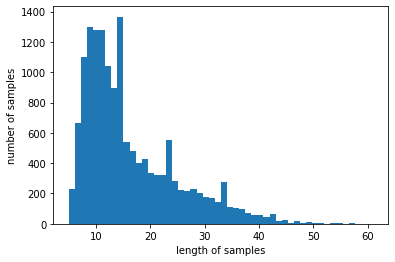
아까 길이가 짧은 애들은 다 날렸었다.
1.3. 워드 임베딩 구축
from gensim.models import Word2Vec

#이번에는 gensim에서 제공하는 Word2Vec 모듈을 사용하여 토큰화 된 네이버 영화 리뷰 데이터를 학습합니다.

embedding\_dim = 100

# initiate the model with 100 dimensions of vectors, 5 words to look before and after each focus word, etc.

# and perform the first epoch of training

model = Word2Vec(
	sentences = tokenized\_data,
	size = embedding\_dim,
	window = 5,
	min\_count = 5,
	workers = 4,
	sg = 0
)

#학습이 완료되었으면, 이번에 구축한 임베딩 행렬의 크기를 알아봅시다!
print(model.wv.vectors.shape) #(5079,100)

#단어 사전에는 총 5079개의 단어가 존재하며, 각각의 단어는 우리가 미리 설정한 embedding\_dim=100 차원으로 구성되어 있음
word\_vectors = model.wv
vocabs = list(word\_vectors.vocab.keys())
vocabs\[:20\]
['평점',
'나쁘다',
'않다',
'짜다',
'리',
'더',
'더욱',
'아니다',
'갈수록',
'개판',
'되다',
'중국영화',
'유치하다',
'내용',
'없다',
'잡다',
'말',
'안되다',
'무기',
'그리다']
gensim 패키지에서 제공하는 most_similar 메소드를 사용하여, 원하는 단어와 유사한 단어들을 찾아봅시다!
for sim\_word in model.wv.most\_similar("마블"):
print(sim\_word)
('시리즈', 0.9973355531692505)
('공포영화', 0.997304379940033)
('드디어', 0.9972233772277832)
('대박', 0.9972142577171326)
('극장판', 0.9970725774765015)
('이제야', 0.9970681667327881)
('잊혀지다', 0.9970123767852783)
('최근', 0.9969878792762756)
('간만', 0.9969663619995117)
('ㅜㅜ', 0.9968585968017578)
for sim\_word in model.wv.most\_similar("슬픔"):
print(sim\_word)
('떠나다', 0.9995038509368896)
('삶', 0.9995024800300598)
('상처', 0.9994688630104065)
('죽음', 0.9994673728942871)
('그것', 0.9994569420814514)
('스스로', 0.9994416832923889)
('만나다', 0.9994298219680786)
('희망', 0.999416708946228)
('불륜', 0.9994130730628967)
('의식', 0.999403715133667)
for sim\_word in model.wv.most\_similar("짜다"):
print(sim\_word)
('이딴', 0.9988716840744019)
('별', 0.9986245036125183)
('알바', 0.9984718561172485)
('점주', 0.9984467625617981)
('마이너스', 0.9984369874000549)
('ㅡㅡ', 0.9984122514724731)
('믿다', 0.9983730316162109)
('말다', 0.9982342720031738)
('별개', 0.9981657266616821)
('인데', 0.9981226921081543)
혹은 similarity 메소드로 단어 간 유사도를 계산해볼 수도 있음
print(model.similarity('슬픔', '눈물')) # 0.99
print(model.similarity('슬픔', '재미')) # 0.96
print(model.similarity('행복', '재미')) # 0.96
2. 한국어 워드 임베딩 시각화
고차원의 벡터를 시각화하기 위해서는 2차원 혹은 3차원으로 벡터를 축소하는 과정이 필요합니다.
2.1. PCA 사용
첫 번째로, PCA라 불리는 대표적인 차원 축소 방식을 사용해볼게요!
from sklearn.decomposition import PCA

import matplotlib.font\_manager

font\_list = matplotlib.font\_manager.findSystemFonts(fontpaths=None, fontext='ttf')
\[matplotlib.font\_manager.FontProperties(fname=font).get\_name() for font in font\_list if 'Nanum' in font\]
['NanumMyeongjo',
'NanumGothic',
'NanumBarunGothic',
'NanumGothic',
'NanumSquareRound',
'NanumSquare',
'NanumSquareRound',
'NanumMyeongjo',
'NanumSquare',
'NanumBarunGothic']
plt.rc('font', family='NanumBarunGothic')

word\_vector\_list = \[word\_vectors\[word\] for word in vocabs\]

word\_vector\_list\[0\]
array([ 0.381261 , 0.3740127 , 0.6019033 , 0.4046414 , -0.46579272,
-0.8931294 , 0.09905372, -0.09076516, -0.57191813, 0.14766434,
0.66556114, -0.6048861 , 0.2438089 , -0.5843505 , 0.31202883,
-0.41703656, 0.05459064, 0.2830779 , -0.23710148, 0.07351534,
0.2686083 , 0.5453253 , 0.12662494, 0.43715692, -0.10033856,
-0.9039592 , 0.6628758 , 0.3481094 , -0.22312832, 0.42010123,
0.36159325, -0.44119486, -0.09792554, 0.31407207, 0.6445948 ,
-0.49734366, -0.5103982 , 0.32681122, -0.20486802, 0.32354006,
-0.04870545, -0.18626834, 0.33107126, 0.32418677, 0.55873215,
-0.27155092, -0.23563509, -0.15540934, 0.17340088, -0.17958516,
0.07491318, 0.6871519 , -0.08649576, -0.1543745 , 0.3377218 ,
-0.34783792, -0.51066256, 0.12337771, 0.08450513, -0.5274035 ,
-0.61068237, 0.13250344, 0.34829745, 0.4433815 , 0.01342276,
0.2567166 , -0.04875081, 0.49946696, 0.87563527, 0.6861587 ,
-0.20344402, 0.2198644 , 0.25345302, -0.335228 , 0.5527798 ,
-0.4047302 , 0.10241615, 0.6993287 , 0.4764856 , -0.30132112,
-0.15017748, 0.3270078 , -0.0354127 , 0.78079593, -0.08559458,
-0.05862745, -0.84043765, 0.21879548, 0.0252186 , 0.70968014,
-0.38477224, 0.42488518, 0.00493145, -0.13044709, 0.12535872,
-0.22751583, 0.3132797 , 0.459829 , 0.12089476, -0.08890179],
dtype=float32)
pca = PCA(n\_components=2)
xys = pca.fit\_transform(word\_vector\_list)

x\_asix = xys\[:, 0\]
y\_asix = xys\[:, 1\]

def plot\_pca\_graph(vocabs, x\_asix, y\_asix):
plt.figure(figsize=(25, 15))
plt.scatter(x\_asix, y\_asix, marker = 'o')
for i, v in enumerate(vocabs):
plt.annotate(v, xy=(x\_asix\[i\], y\_asix\[i\]))

plot\_pca\_graph(vocabs, x\_asix, y\_asix)
결과를 보면, 많은 벡터들이 한 곳에 모여있기 때문에 임베딩의 품질을 제대로 확인할 수 없습니다.
2.2. t-SNE 사용
앞서 사용한 PCA가 자주 이용되는 차원 축소 방식이긴 하지만, PCA는 군집의 변별력을 해친다는 단점이 있음
이를 개선한 방법이 t-SNE 차원 축소 방식으로 이번에는 t-SNE 방식으로 차원을 축소해볼게요!
from sklearn.manifold import TSNE

tsne = TSNE(learning_rate = 100)
transformed = tsne.fit_transform(word_vector_list)

x_axis_tsne = transformed[:, 0]
y_axis_tsne = transformed[:, 1]

def plot_tsne_graph(vocabs, x_asix, y_asix):
plt.figure(figsize=(30, 30))
plt.scatter(x_asix, y_asix, marker = 'o')
for i, v in enumerate(vocabs):
plt.annotate(v, xy=(x_asix[i], y_asix[i]))

plot_tsne_graph(vocabs, x_axis_tsne, y_axis_tsne)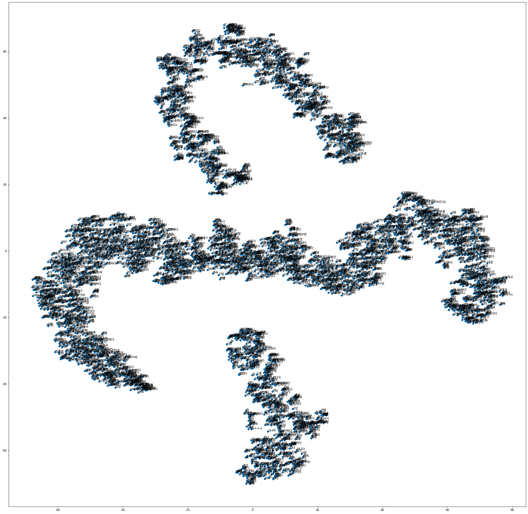
2.3. t-SNE 고도화
여전히 눈으로 확인하기 어려운데요,
Python에서 제공하는 interactive visualization library인 bokey를 사용하여 t-SNE를 보기 좋게 시각화해볼게요!
import pickle

tsne_df = pd.DataFrame(transformed, columns=\['x_coord', 'y_coord'])
tsne_df

tsne_df\['word'] = vocabs
tsne_df

from bokeh.plotting import figure, show, output_notebook
from bokeh.models import HoverTool, ColumnDataSource, value

output_notebook()

# prepare the data in a form suitable for bokeh.

plot_data = ColumnDataSource(tsne_df)

# create the plot and configure it

tsne_plot = figure(title='t-SNE Word Embeddings',
	plot_width = 800,
	plot_height = 800,
	active_scroll='wheel_zoom'
)

# add a hover tool to display words on roll-over

tsne_plot.add_tools( HoverTool(tooltips = '@word') )

tsne_plot.circle(
	'x_coord', 'y_coord', source=plot_data,
	color='red', line_alpha=0.2, fill_alpha=0.1,
	size=10, hover_line_color='orange'
)

# adjust visual elements of the plot

tsne_plot.xaxis.visible = False
tsne_plot.yaxis.visible = False
tsne_plot.grid.grid_line_color = None
tsne_plot.outline_line_color = None

# show time!

show(tsne_plot);
2.4. 임베딩 프로젝터 활용
조금 더 interactive한 분석을 위하여, 이번에는 임베딩 프로젝터(embedding projector)라는 Google이 제공하는 데이터 시각화 도구를 사용하여 우리가 학습한 임베딩 행렬을 시각화하고, 분석해봅시다!
https://projector.tensorflow.org/
from gensim.models import KeyedVectors

model.wv.save_word2vec_format('sample_word2vec_embedding')

!python -m gensim.scripts.word2vec2tensor --input sample_word2vec_embedding --output sample_word2vec_embedding
이제, Embedding Project 사이트에 들어가서, tensor.tsv, metadata.tsv 파일을 업로드합니다.
글씨가 많이 깨졌네요 ...
역슬레쉬는 다 지우고 사용하면 됩니다...
'인공지능 > 자연어 처리' 카테고리의 다른 글
| 자연어 처리 문장 임베딩 만들기 - Seq2Seq (1) | 2024.03.24 |
|---|---|
| 자연어 처리 문장 임베딩 만들기 - 자연어 처리를 위한 모델 구조 (0) | 2024.03.24 |
| 자연어 처리 python 실습 - 한국어 Word2Vec 임베딩 만들기 (0) | 2024.03.17 |
| 자연어 처리 python - 워드 임베딩 만들기 - GloVe (0) | 2024.03.17 |
| 자연어 처리 python - 워드 임베딩 만들기 - Fast Text (0) | 2024.03.16 |